Experimental Investigation of Vortex-Tube Streamwise-Vorticity Characteristics and Interaction Effects with a Finite-Aspect-Ratio Wing


Department of Mechanical Engineering, North Dakota State University, Fargo, ND 58108, USA
*
Author to whom correspondence should be addressed.
Fluids 2020, 5(3), 122; https://doi.org/10.3390/fluids5030122
Submission received: 16 June 2020
/
Revised: 17 July 2020
/
Accepted: 22 July 2020
/
Published: 24 July 2020
(This article belongs to the Special Issue Particle-Based Simulation of Fluid Dynamics)
Abstract
:An experimental study is conducted to analyze a streamwise-oriented vortex and investigate the unsteady interaction with a finite-aspect-ratio wing. A pressurized vortex tube is used to generate streamwise vortices in a wind tunnel and the resulting flow behavior is analyzed. The vortex tube, operated at various pressures, yields flows that evolve downstream under several freestream wind tunnel speeds. Flow measurements are performed using two- and three- dimensional (2D and 3D) particle image velocimetry to observe vortices and their freestream interactions from which velocity and vorticity data are comparatively analyzed. Results indicate that vortex velocity greater than freestream flow velocity is a primary factor in maintaining vortex structures further downstream, while increased supply pressure and reduced freestream velocity also reduce vortex dissipation rate. The generated streamwise-oriented vortex is also impinged on a finite-aspect-ratio airfoil wing with a cross-section of standard NACA0012 airfoil. The wingtip-aligned vortex is shown to investigate the interaction of the streamwise vortex and the wingtip vortex region. The results indicate that the vorticity at the high vortex-tube pressure has a significant effect on the boundary layer of airfoil.
1. Introduction
Swirling and vortex flows are encountered in many nature and technology applications [1] ranging from formation flights [2,3] to spray and combustor mixing devices [4]. Formation flight, like that observed from birds to improve aerodynamic efficiency [2], is a commonly used technique in groups of aircraft to improve fuel efficiency [3]. In order to improve upon the benefits obtained through formation flight, an understanding of the underlying physical phenomena is necessary. The primary factor in effective formation flight is the alignment of aircraft wings such that the wingtip vortices produced by a leading aircraft will intersect with the wing of a trailing aircraft in a way that increases lift and reduces drag. This intersection has been modeled numerically [5] to produce valuable information about the nature of the fluid flow resulting from the interaction of the wingtip vortex with the trailing wing. In order to verify such numerical methods, a robust real-world approach is needed to allow control over the flow parameters specified in simulations, and the device developed in this study is intended to provide an approach for such control. Therefore, the goal of this research is to develop a method of producing controllable streamwise vortex structure that can be characterized and that can also be used in several applications of swirling flows, such as the experimental analysis of vortex interactions with airfoils. The resulting experimental data can also be used to perform numerical simulation validations. In addition, the canonical nature of the experimental framework permits application to methods for improvement on aircraft performance, such as those using winglets [6], flow control devices such as tubercles [7], etc.
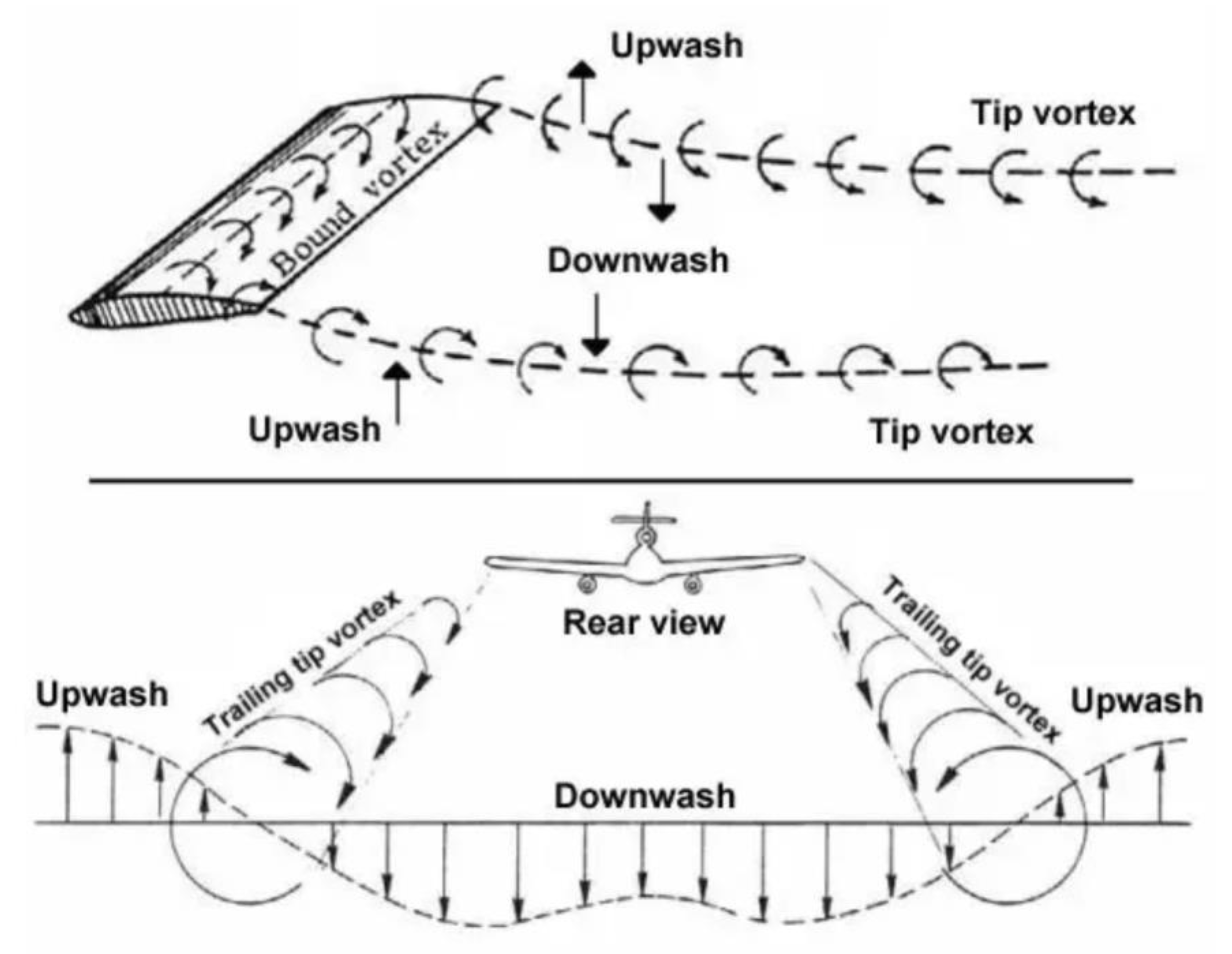
Streamwise vortices are produced during the general operation of finite airfoil wings [8]. The 3D nature of aircraft wings results in increased complexity of the surrounding airflow compared to that of a theoretical 2D airfoil. The high-pressure region created underneath the wing is responsible for producing lift; however, near the wingtips this pressure causes the air to be forced upwards and over the wing. The motion of this air produces a circulatory flow pattern that trails after the wing, known as a wingtip vortex [8]. The air that has circulated to the top of the wing now affects the wing’s upper surface, producing a downward force in a process known as downwash, which reduces the effective angle of attack of the wing [9]. Conversely, the circulating air can also produce an upwards force, known as upwash, before it reaches the upper surface of the wing; however, since the axis about which the air is circulating is aligned with the wingtip, this upwash generally does not affect the wing generating the vortex [10]. The distribution of forces due to vortices is shown in Figure 1 [11]. To reduce the effects of downwash and increase flight efficiency, some aircraft utilize wingtip devices to alter the behavior of the circulating air [6,10]. While theorized prior to its first application, this approach was first implemented by Whitcomb in 1976 by adding nearly vertical wing-like plates known as winglets to the wingtips of aircraft [6,11,12]. The addition of wingtip devices increases the weight of the aircraft and causes increased drag due to the increase in surface area, but the benefits of increased fuel efficiency and maximum range often justify the decision. Wingtip devices may also be used to reduce takeoff noise and increase cruise altitude and speed [6,11,12].
Wingtip vortices produced by finite airfoil wings can impact the flight characteristics of other aircraft. The vortices produced from the wingtip expand in diameter as they trail behind an aircraft [10]. Known also as wake turbulence, these vortices are produced during flight as well as during take-off and landing and have the potential to interfere with the operation of other aircraft with which they come into contact. An aircraft entering wake turbulence may experience sharp sudden aerodynamic moments that can be difficult to recover from. The National Transportation Safety Board (NTSB) records that in the United States between 1983 and 1993, at least 51 incidents and accidents occurred that were most likely caused by the interaction of aircraft with wake turbulence, some of which resulted in the death or injury of aircraft occupants or damage or destruction of one of the aircraft involved. To avoid incidents such as these, the FAA mandates that aircraft remain at a great enough distance away from the wake of other aircraft according to their weight classification, as larger aircraft produce stronger wakes [13].
In a more useful situation, aircraft and birds flying in formation can take advantage of wingtip vortices to increase the lift produced by their wings and improve their efficiency. The technique of formation flight is demonstrated by many species of birds: by flying in a V-shaped pattern, the wingtip vortices produced by the leading bird produce upwash, the opposite effect of downwash, on the trailing birds’ wings when they are located within the upward-moving portion of the wingtip vortex [2]. This upward component of the circulating air creates additional lift and thereby increases flight efficiency. A theoretical examination of this technique showed that the range of a flock of 25 birds would increase by 71% due to the benefits of upwash in formation flight [2]. Similarly, for fixed-wing aircraft, the upwash of a leading aircraft may be used to provide additional lift for other aircraft, increasing efficiency and reducing fuel consumption [14].
Streamwise vortices are also sometimes induced on the surface of an aircraft wing in order to delay boundary layer separation and improve fuel efficiency. These vortex generators are comprised of small fins mounted perpendicularly on the top surface of an aircraft’s wings, at an angle to the incident airflow. As the vortices produced by the fins travel over the surface of the wing, they carry away some of the wing’s slow-moving boundary layer and so delay the separation of the flow over the airfoil. This interruption of flow separation events can be found in the numerical simulations of Garmann and Visbal [5].
In this study, particle image velocimetry (PIV) using its tomography version technique was applied to study the streamwise vortex that is generated in a vortex tube [15] that is controlled by a compressed air with varying inlet pressures and released to various wind tunnel freestream velocities. Then, the controllable generated streamwise vortex with various strengths and endurances was studied and it was also allowed to impinge on a finite airfoil wing to study the interaction with wingtip flow. Besides the fundamental nature of the investigation, it is noteworthy to mention again that there are multiple practical applications of this work that relate to the improvement of aerodynamic efficiency of aircraft using involving vortex surfing [3], winglets [6], etc., and it also relates to multiple other fundamental and applications of swirling flows, such as those common in sprays and combustors [4], etc.
2. Experimental Setup
2.1. Pressurized Vortex Tube
The method used for vortex generation was a pressurized vortex tube. This device circulates compressed air in a cylindrical chamber and then releases the air into the freestream flow. These devices are used in industry to produce separate streams of higher and lower temperature air from a single supply [15]. The device’s operation is illustrated in Figure 2 below. Compressed air is introduced into the chamber from a tangential port near the front of the chamber’s interior. The tangential airflow then circulates along the length of the device, and upon reaching the end of the chamber the central portion of the vortex air is reflected back through the chamber to exit the front of the device, while the heated outer air is released through a valve at the back end. In this study, the valve is removed entirely to allow the air to continue its circulatory pattern outside the device, forming a streamwise vortex. This approach allows for the strength of the produced vortex to be manipulated by increasing or decreasing the pressure of the compressed air supplied to the vortex tube.
The pressurized vortex tube was constructed by 3D printing with ABS plastic with a cylindrical chamber length of 6 inches, an internal diameter of 0.25 inches and an external diameter of 0.375 inches. The tangential inlet had an internal diameter of 0.0625 inches and was supplied with compressed air through 0.036 inch ID tubing. The dimensions of the device were chosen to conform to the vortex size relations imposed by the numerical simulation of Reference [5]: streamwise vortices with an outer diameter of 0.25 inches corresponds to an airfoil chord length of 1.25 inches, and for an aspect ratio of 6 this airfoil would have a wingspan of 7.5 inches. As a result, the wingtip of the airfoil of corresponding size would be located near enough the center of the 12 in2 wind tunnel test section, with the goal of sufficient spacing to avoid interacting with the boundary layers on the wind tunnel walls and other wind tunnel interferences [16,17,18,19,20,21,22]. Both ends of the chamber were left open in the initial design of the part to allow future testing to investigate the effects of allowing the freestream flow to enter the chamber, but the front end of the chamber was sealed during testing. To determine the effects of changes in air supply pressure on the produced vortices, the device was operated with supply pressures of 20, 30 and 40 psi which translate into the flow conditions of Table 1. The device is pictured in Figure 3 below, mounted on a slider system to allow spanwise motion for transient tests and in a typical wind tunnel mounted configuration with various dimensions of interest.
2.2. Wind Tunnel
Tests were conducted inside a FloTek 1440 wind tunnel with a test section area of 12 in2 that was operated at various speeds for each vortex generation apparatus. For each configuration of each vortex generator, the wind tunnel was operated at speeds ranging from 3% to 43% of the full power speed for the 2-dimensional (2D) PIV tests, and from 3% to 20% of the full power speed for 3-dimensional (3D) tests. The corresponding freestream velocities were then determined for each wind tunnel percentage using separate Pitot tube and freestream PIV measurements obtained prior to testing, with the results shown in Table 1 (where WT means wind tunnel and VT vortex tube). The percentages used in the various conditions reported in the investigation refer to the freestream and Reynolds number conditions of the table. The rest of experimental conditions related to the vortex tube flow are also shown in the table for the exit flow and were obtained from the PIV campaigns in the manner described in the results section. The Re number for the vortex flow is obtained from the tube exit magnitude of velocity at each condition (Uo) the tube inner diameter (0.25 in or 6.35 mm) (d), and the air kinematic viscosity (ν) at 15 °C (1.48 × 10⁻⁵ m2/s) as Re = Uo × d/ν. The table quantities enlighten the fact that the flow is indeed 3D at the exit, having high tangential components.
Wind tunnel testing, especially when directed towards validation of numerical simulations, brings up a series of concerns that need be addressed properly and scaling considerations and boundary conditions corrections have to be considered. These concerns include the influence of Reynolds and Mach numbers, the scaling quality and accuracy, the wall-interference effects, the flow and solid blockages, the freestream turbulence, etc. [16,17,18,19,20,21,22]. Investigations have clearly concluded that corrections for aerodynamic coefficient measurements (notably lift and drag) have to be properly used to represent the natural flow conditions encountered by models. These corrections come about from the fact that wall separations and boundary layer developments interfere with the model natural flow conditions sought for the engineering assessments. It is thus obvious that the current testing will be affected by such wind tunnel interference and, indeed, wind tunnel freestream and wall flow interrogation and calibrations performed with pressure probes and PIV revealed irregularities that would have to be considered when measuring flows and airfoil properties. For the purposes of this investigation, which concerns streamwise vorticity of various levels and its impingement on an end tip of an arbitrary and thin airfoil centered in the test section, these corrections were less critical than studies on aerodynamic performance such as lift and drag. In this study, irregularities were observed very near to the test section walls and were avoided by placing the vortex generator in the center of the test section to ensure a uniform freestream flow during testing. As previously discussed, avoiding the effects of the irregularities was also a factor in selecting the dimensions of the vortex tube. It is nonetheless clear that the strength, evolution and interactions of the vorticity generated in the wind tunnel would differ from those in a natural “free” environment and further studies would be needed to assess the differences.
The freestream velocity coupled with the vortex tube flow exit was responsible for carrying the streamwise vortex away from the generator, and as such an increase in freestream velocity would affect the periodicity of the vortices. This was a contributing factor to focus on lower speed setting tests for both 2D and 3D PIV to assess streamwise vorticity strength, evolution, and interaction with a downstream object, such as a wing [5].
2.3. Particle Image Velocimetry (PIV) Setup
The vortices produced by the generation apparatus were observed using both 2D and 3D PIV approaches [23,24] for the various tunnel conditions. For the PIV system, the schematic of the system used in the present study and photography of the laser sheet path, the four-camera PIV setup, and the particle seeding system are shown in Figure 4 along with schematics showing the laser illumination used for the data acquisition campaigns.
Small droplets of sub-micron diameter were introduced into the wind tunnel as an aerosol produced from atomization of DEHS oil. Pressurized air is injected into a tank of this oil, producing droplets around air bubbles. The oil−air mixture is then carried to the diffusors where it is released as a mist into the inlet of the wind tunnel. Due to their small size, gravitational and inter particle forces are ignored, and these droplets are characterized as accurately following the flow path of the airflow inside the wind tunnel. The density of the mist released into the wind tunnel was controlled by modifying the pressure of the supplied air to ensure that the proper particle density was present during testing. Not enough particles in the flow would prevent accurate measurements from being obtained, while too many particles would lead to excessive computational effort being required to process the resulting images.
The droplets were then illuminated by a double-pulsed Nd:YAG laser (NewWave MiniLase-III) capable of emitting two laser pulses of 100 mJ at a wavelength of 532 nm with a repetition rate of 30 Hz, as shown in Figure 4. For 2D PIV, the laser was expanded into a vertical sheet parallel with the flow using spherical optics, which was centered at the axis of the vortex generator. For tomographic PIV, the laser was expanded to shine over a volumetric region of interest for the apparatus, with thickness of 10 mm set by a rectangular aperture, and specifically over the flow region immediately following the outlet of the vortex tube (Figure 4e) and downstream regions such as the wingtip of the airfoil (Figure 4f). For the study of the vortex−airfoil interaction, the vortex tube was held vertically to minimize obstruction on the flow from the vortex tube holder on the horizontal airfoil (Figure 4f). The dimensions of this region remained unchanged between tests to allow comparison of the data between configurations without needing to account for differences in location of the test volume.
For each measurement instance, the laser emits two pulses separated by less than 100 μs to illuminate the region and capture two images of the particles with appropriate displacements expected at the magnification and flow dynamic ranges. A timing interval for the pulses is selected that is short enough that the displacement of the particles is small enough for the correlation algorithm to identify the individual particles’ positions in both frames, but also large enough that the difference of the particles’ positions is great enough to produce optimal accuracy measurements [23,24,25]. When chosen properly, the resulting vectors obtained from the measured displacement and time provide an effectively instantaneous velocity field of the observed flow region.
The selection of this interval is complicated by the presence of multiple flow regions with varying velocities; in such a flow, the proper interval may be suitable for a slower flow but unable to accurately measure the faster flow region, or vice versa. This problem limited the velocities that could be tested in the wind tunnel, as even at the 43% setting the difference between the freestream velocity and vortex velocity made accurate measurement more difficult, so data collection was focused on lower speeds for this investigation. The selected 2D timing intervals for each configuration were set from 30 to 60 μs depending on the vortex tube flow and freestream conditions.
Images of the illuminated droplets were then captured using Charged-Coupled-Device (CCD) PIV double-frame cameras with 1600 × 1200 resolution mounted outside the tunnel at various positions and angles. These cameras are designed to rapidly capture two images corresponding to the two laser pulses in each measurement instance.
During 2D operation, the cameras captured images spanning approximately 40 mm (1.575 inches) in the x-direction and 30 mm (1.181 inches) in the y-direction, while the tomographic camera arrangement, as shown in Figure 4 above, captured images in their own local coordinate systems. For tomographic operation, the resulting images were used to reconstruct the 3D positions of the droplets within the flow region of interest in both frames. For both 2D and 3D approaches, a cross-correlation algorithm was applied to the two consecutive frames to identify the displacement of the particles between frames [23,24,25].
As previously mentioned, these displacement vectors, when divided by the time interval between frames, produce effectively instantaneous 2D (u, v) or 3D (u, v, w) velocity fields of the flow for individual camera views or tomographic reconstructions, respectively. Further related details of these techniques as well as other vortex generation designs considered for this investigation can be found in [26].
3. Results
The pressurized vortex tube was tested first using 2D PIV to verify the device’s operation and to determine the extent to which the produced streamwise vorticity could be maintained downstream. One camera was placed parallel to the flow viewing the region around the outlet of the device and another in a similar orientation to observe the region immediately downstream of that of the first camera. This allowed the degree of dissipation of the vortices streamwise vorticity to be observed after they had travelled a fixed distance. Although the 2D renderings in the streamwise plane are useful and yield a first impression and guidance of the vortex flow main location and quality, it is obvious that only a 3D flow field from the tomographic PIV is expected to render a full characterization of the complex flow. In keeping up with this philosophy, initial developments, flow features, vortex main spanwise locations, skewness and direction, etc., will be easily drawn from the 2D data and then the 3D data will be collected in the regions found of interest and presented to complement the findings.
The results will show flow properties derived from the PIV velocity field including streamlines, vorticity, and other means to find vortex core regions [27,28,29], such as iso-surfaces of Q-criterion [27]; both instantaneous and average renderings will be utilized to highlight the unsteady nature of the flows. The data cover downstream regions from the outlet of the vortex tube and they are organized to show characteristics as a function of the settings of the vortex tube pressure, that determines the vortex strength, and the wind tunnel speed, that determines the freestream condition, at which each dataset was obtained; they are arranged to display the different conditions together and allow their direct comparison and analysis. Since a small portion of the vortex tube was visible within the near camera frame during data collection, approximately 12 mm2 (0.0186 in2) of invalid or missing data is present where the overlap occurred, centered at the vertical location of the outlet y = 0. All numerical data have been presented at the same scale as data of the same type.
For every case, several figures are presented first to show instantaneous data choosing the median frame of the set (a robust statistic [30]) as the illustrative representation in their associated datasets. In the streamline graphs, 300 random points were used to generate the streamlines and are colored with velocity magnitude. Then, the following figures present the time-averaged data from the same datasets. The downstream 2D camera view data are organized similarly in the figures. Following the instantaneous snap samples, the averaged flow fields presented yield a representation of the flow’s average patterns for the various conditions.
It is important to note that the maximum repetition rate at which the laser could operate (30 Hz) was too slow to capture time-resolved particle image data from the vortex structures, since they manifest and travel at smaller timescales than the PIV apparatus is capable of operating at. Thus, time averaging the vorticity data could not produce meaningful results due to this timescale issue as well as the turbulent nature of the vortices, and instead only the instantaneous vorticity data are presented. It is also important to note that the vorticity maps from the 2D images present the vorticity in the z-direction, i.e., negative normal to the camera, since only x and y data are available in these images.
As discussed in the aforementioned experimental setup section, in order to correctly perform the correlation calculations, the time interval between two consecutive frames (‘dt’) must be small enough to observe the flow particles with a small but still measurable displacement. This leads to difficulty in obtaining accurate measurements when observing a slow-moving vortex core in a high-speed freestream flow, or a high-speed vortex core in a slow-speed freestream flow. In this study, observation of the vortex was prioritized and a value for ‘dt’ was selected to ensure accurate measurement of the vortex core as explained in the previous section. This value is shown in each of the individual graphs in the Figures.
3.1. 2D Velocity Maps, Vectors and Streamlines
Several results are immediately apparent from the instantaneous 2D data. The velocity and streamline graphs indicate that the vortices entrain the freestream flow to a much greater extent when the difference in velocity between the vortex core and freestream is large due to the larger difference in the mixing layer between the vortex flow and the freestream flow [31,32,33,34]. The complex three-dimensional events involve mixing streams with velocity gradients and they evolve downstream to display free-shear turbulent flow characteristics [35] after the internal vortex-tube complex developments [36,37,38].
This is most evident in the 40 psi and 3% wind tunnel setting, for which the velocity map is presented below in Figure 5a. In this configuration, near the outlet of the vortex generator, the majority of the vortex possesses a velocity approximately 20 m/s faster than the surrounding flow. The corresponding streamlines for this configuration are shown in Figure 5b, where it can be clearly seen that the freestream is entrained into the vortex due to the significantly higher velocity of the vortex structure. In contrast, the velocity map and streamlines from a configuration with similar velocities in the freestream and vortex structures shows that entrainment is greatly reduced when the vortex structure velocity is greater than the freestream velocity, but this difference in velocity is small. A prime example of this is the 20 psi vortex tube and 20% wind tunnel settings, shown in Figure 5c. In this configuration, the freestream flow is only slightly influenced by the presence of the vortex structure, as evidenced by the corresponding streamlines presented in Figure 5d. While it may also be inferred that high-speed flows generally entrain the vortices in smaller scales than flows at lower speeds, this hypothesis is complicated by the varying degree of entrainment of freestreams by the vortices at different pressure settings.
The colored streamline plots are additionally useful because they clearly convey the fact that the flow is 3D. This is indicated with areas with higher and lower velocities through the given streamlines (which are tangents to the projections of the 3D vectors in the 2D plane) and imply a divergence (and a w component) in the plane (another indication of three-dimensionality). This is discussed further in the tomographic data analysis section.
Additionally, several small vortices and circulation areas in the xy-plane can be seen throughout the vortex structure in Figure 5, primarily in the upper portion of the graph, which may indicate the location of an annular portion of the vortex structure perpendicular to the camera, i.e., with its centerline extending in the z-direction. Additionally, present to varying degrees in the corresponding vorticity maps, these circulation regions also appear frequently in the other 2D and 3D streamline graphs, most obviously in the 30 psi and 20% setting streamlines shown in Figure 6, which indicate the presence of an annular structure formed immediately after the outlet of the vortex generator.
As expected, from the velocity maps it can be observed that the vortices are rotating more quickly at higher pressures, since both the top and bottom of the vortex structures are more visible in the instantaneous data from configurations with 40 psi settings.
The downstream vortex tube test is of importance for characterizing vortex developments and also for establishing a frame of reference for the flow that will be interacting with the airfoil later. A few representative results are shown in the following sections. Due to a smudge or dirt on windows on the laser sheet path, a small linear distortion is visible in nearly all velocity datasets at approximately x = 35 mm (1.378 inches), and another small distortion centered near x = 30 mm (1.181 inches), y = −7 mm (−0.276 inches) is also visible in the vorticity data. Most notable in these datasets is that the vortex structures remain intact further downstream for configurations in which the exit velocity of the vortex tube is much larger than the freestream velocity. In both the instantaneous and time-averaged velocity maps, the vortices produced at the 20 psi pressure setting have largely dissipated before entering the frame of the downstream camera, whereas at the 40 psi pressure setting the central region of the vortices are still clearly visible. However, the downstream vortices maintain their average velocity for longer at the 20% setting. In the instantaneous downstream data, the turbulent nature of the vortices is more noticeable than in the near camera view data. As previously discussed in this section, since the camera timing is not synchronized to the period of the vortices, the motion of the vortex structures cannot be followed frame-by-frame. However, the instantaneous images still show the vortices at various orientations as they spiral downstream, as will be shown in downstream datasets and that can be found in the full dataset in [26]. It is observed that the 2D vector field does not reflect clearly that motion due to the 2D limitations in a 3D flow and that tomographic results are needed.
Most enlightening developments can be traced once the data for the various wind tunnel speeds and vortex pressures are put together side by side as shown and discussed next using representative instantaneous samples (Figure 7) and averages (Figure 8) of velocity contour maps in the near field. The instantaneous maps first revealed the turbulence nature of the vortex flow, clearly characterized by strong fluctuations and jitter among realizations that are typical of free (unbounded) turbulent flows [35]. To this point, as alluded earlier, mention needs to be made to the fact that the vortex tube, where the vortex is generated, is a complex geometry with a confined boundary, a free end, and lengthy internal boundary conditions; it also houses an interaction with the other swirling cold vortex flow and with an exit flow and the mixing flow with the free stream environment. Studies with even simpler geometries have revealed unstable flow patterns quickly developing and depending on several geometric and swirl flow parameters [36,37,38]; these studies have also depicted flow patterns once the vortex is generated, becomes unstable upon freestream interaction and mixing (a complex 3D spiraling mixing layer phenomena), and produces vortex breakdown phenomena [5,31,32,33,34,39,40]. As depicted in the data that follows, the vortex is typical of an unsteady turbulent swirling vortex flow.
The swirling flow coming out from the vortex tube starts mixing with the free stream at the various ratios and it is clear and expected that as the ratio of the velocities decreases from an almost quiescent free stream (3% wind speed) to the higher velocities, the mixing region becomes thinner as illustrated in the instantaneous (Figure 7) and averaged (Figure 8) data plots. The instantaneous samples reveal individual structures, for example, those centered at the higher velocity spots (e.g., those in the frame corresponding to 40 psi and 10% wind speed), that were detected in the streamlines shown earlier, and that will be further and better demonstrated with vorticity maps. They also show a tendency of the main vortex flow location to be slightly skewed downwards for the high pressure vortex conditions, an asymmetric feature related to the specific orientation of the vortex tube inlet, that tends to vanish as the vortex strength (pressure) is lower. The average maps corroborate this main pattern with two prominent “jets” at this 2D plane. The sudden disappearance of these “jets” some short distance downstream is indeed a signature of the three-dimensional swirling nature of the vortex.
The downstream flow follows the trend that the stronger and more lasting vortex is indeed that with the higher pressure setting (40 psi), as demonstrated by few sample conditions for instantaneous (Figure 9) and average (Figure 10) velocity maps. Further samples and other conditions can be found in [26]. As mentioned earlier, these downstream flows are as crucial as the ones that will produce the interaction with the downstream airfoil.
The vorticity in the x-direction cannot be observed in 2D testing in which the cameras are facing the negative z-direction, but z-vorticity data can still be used to draw conclusions about the flow behavior. Figure 11 shows the z-vorticity map from the near camera from the 40 psi and 5% configuration, the velocity map of which was shown in Figure 7. In this near map it can be seen that the regions with high-magnitude z-vorticity correspond to the high-velocity regions from the outlet of the vortex generator as seen in Figure 7. In particular, the location of the region centered at approximately (0, 3) mm or (0, 0.118) inches in Figure 11 matches part of a high-velocity region in Figure 7. This vorticity is likely produced by a previously discussed annular portion of the vortex structure. The interaction of the vortex flow with the freestream leads to mixing layers with vorticity of opposite signs as seen in the Figure. These 2D vorticity maps have strong limitations and, thus, 3D tomographic mapping is needed for the full characterization of vorticity fields, as will be shown in the following section.
3.2. 3D Tomographic Test Results Overview
After the initial assessment with the 2D PIV campaign, where the main regions of interest for vorticity activity were identified, tomographic testing was performed to observe the vortex structures with more detail. Since the tomographic approach only allows for a limited span (z axis) of area to be observed, the available PIV hardware apparatus was focused on the outlet region, and further downstream behavior of the vortices was not observed simultaneously. The vortex generator was operated in the same configurations as with the 2D analysis, and the laser apparatus was modified to illuminate a 70 mm (2.755 inches) long, 10 mm (0.398 inches) thick and 50 mm (1.969 inches) tall volume immediately following the outlet. Four PIV cameras were then positioned to observe this region from multiple orientations to produce the images to be used for tomographic reconstruction, as shown in Figure 4. It is important to note that the orientation of the vortex tube in the wind tunnel causes the produced vortex to have a positive vorticity in the x-direction.
The tomographic data are plotted and grouped to allow direct view and comparison of the various conditions, wherein the vortex behavior is much more clearly visible than in the 2D datasets. As with the 2D data, the 3D instantaneous data are shown for the median camera frame followed by the time averaged data. Additionally shown are the instantaneous Q-criterion isosurfaces [27] for the median camera frame colored by velocity magnitude. The instantaneous velocity vectors show the circulatory motion at several planes along the length of the tomography volume much more readily than the 2D views. These also further support the conclusion that when the vortex velocity is greater than that of the freestream, the difference in velocity between the vortex and freestream is the primary factor in maintaining the vortex structures in the flow. Note that the locations of the planes at which data are presented are constant for all graphs.
After completing this analysis, a final set of tomographic tests was performed to observe the interaction of the vortices with a NACA 0012 airfoil with an aspect ratio of AR = 4 and an angle of attack of 5°. This test allowed both the study of the influence of having higher turbulence on the airfoil as well as the influence of strong streamwise vorticity in the freestream from the various conditions. The airfoil was placed 6 inches downstream from the vortex tube to prevent the wake from the generator apparatus from interfering with the vortex−airfoil interaction. The vortex generator was positioned at the same elevation as the airfoil, and slightly offset from the wingtip such that the outside of the vortex tube was tangent to the vertical plane of the airfoil wingtip. While not ideal for detecting wingtip vortex dissipation, this was done to allow the laser to be projected on the upper surface of the airfoil rather than on the wingtip. Centering the laser volume over the wingtip would have caused the edge of the airfoil to produce significant glare in each of the tomographic camera views, which was avoided by moving the laser volume slightly spanwise inward over the airfoil such that the edge of the airfoil was just outside the laser volume. Due to the orientation of the laser, only data from above the airfoil could be obtained, and additional measurement apparatus or an alternative setup would be required to measure both the top and bottom surfaces. While insightful, these tests were primarily intended to demonstrate the capability of the vortex generator rather than produce a sizable dataset to work with, and additional testing will be required to fully verify the results of the numerical simulations, such as those in [5].
3.3. 3D Tomographic Data Analyses
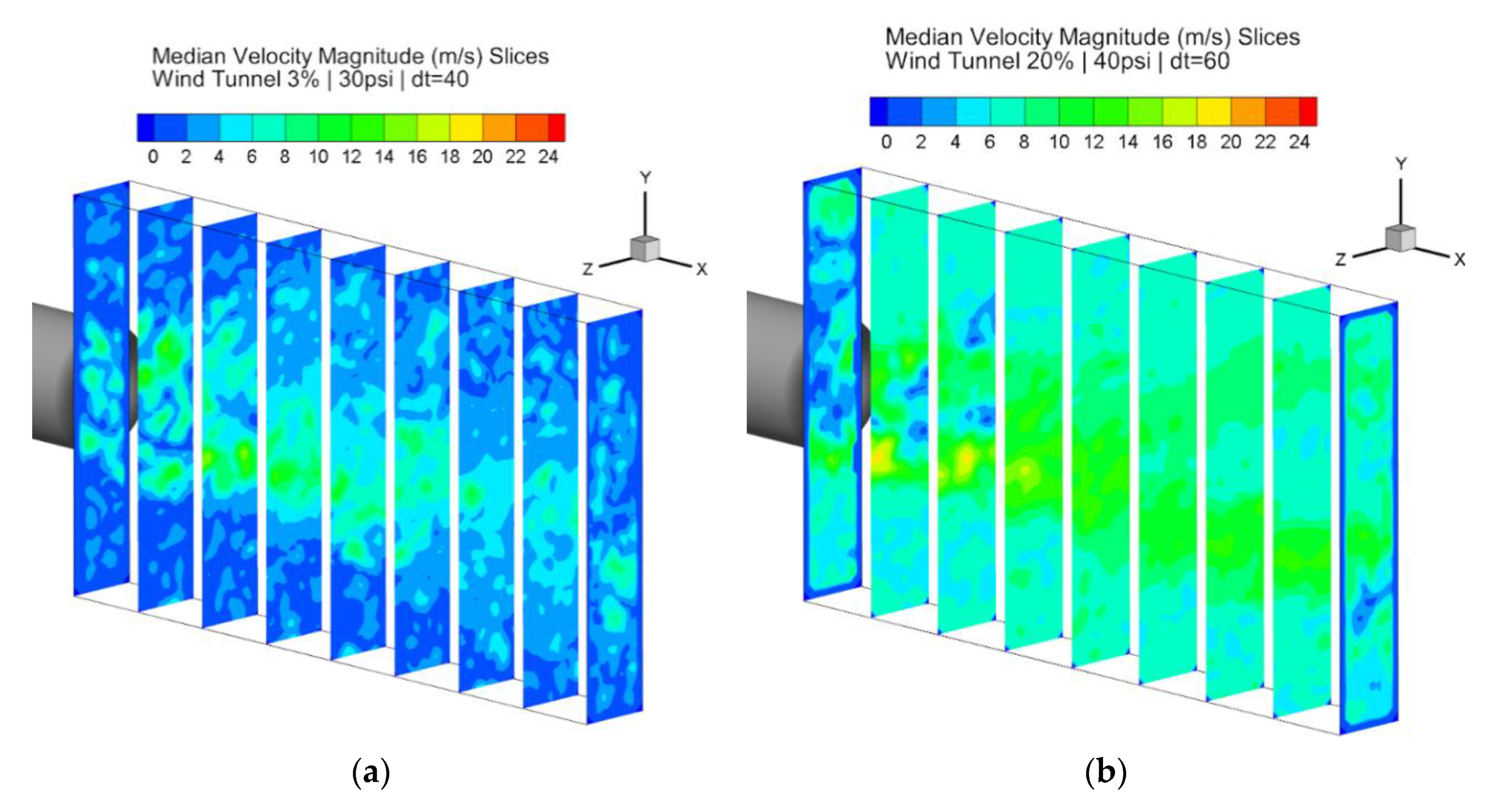
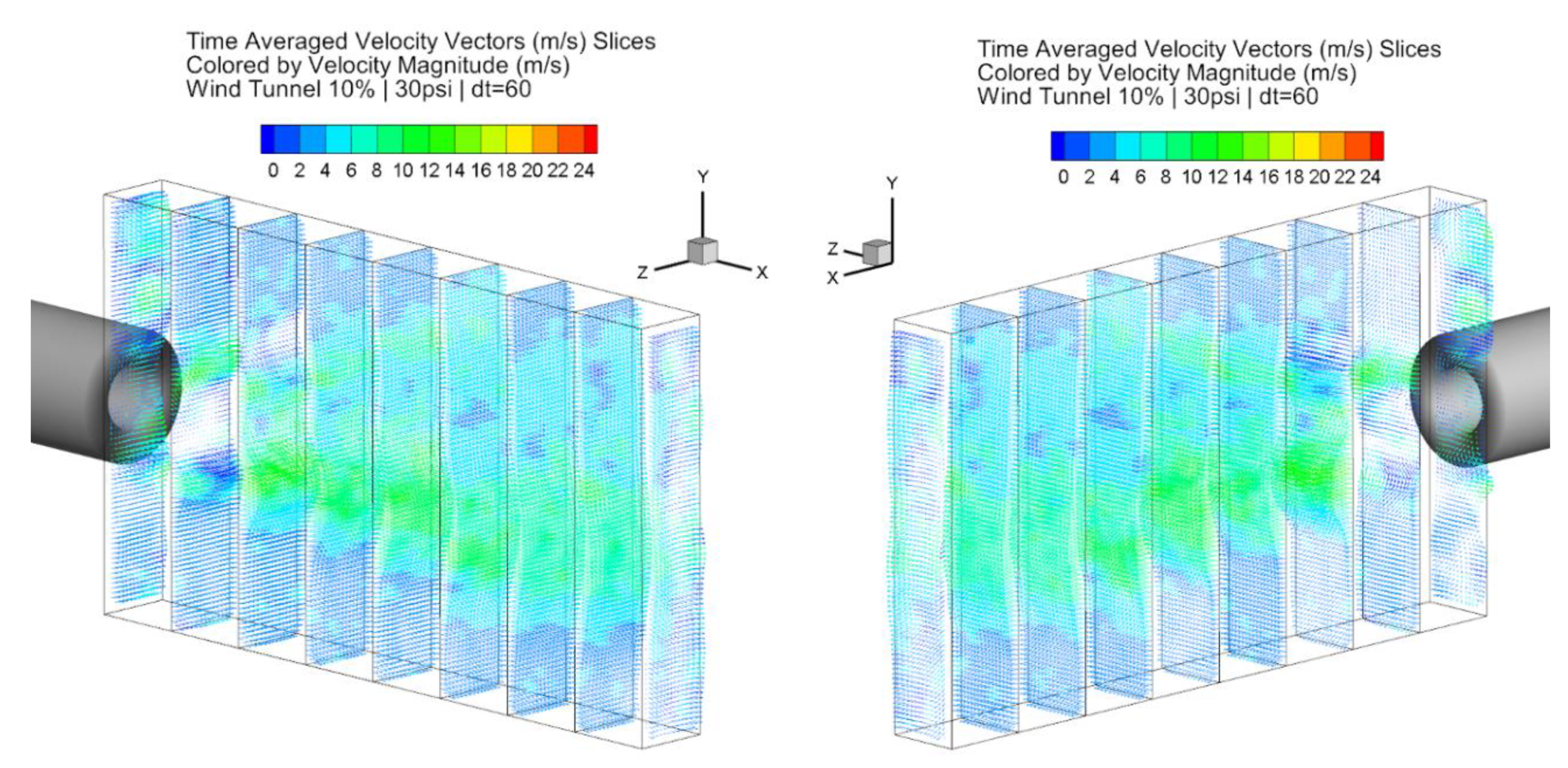
A prime example of the aforementioned significance of velocity difference and three-dimensionality is the contrast between the graphs of instantaneous velocity vectors with changing wind tunnel and vortex pressure settings. Figure 12 shows such examples for a wind tunnel set to 3% and the vortex tube operating at 20 psi (Figure 12a) versus 40 psi (Figure 12b), and for the vortex pressure of 20 psi interacting with the freestream generated from the wind tunnel set to 5% (Figure 12c) versus 10% (Figure 12d). The insightful addition of the third dimension, making the vector plots appear flooded with spatial data, is indicative of high activity in the three spatial dimensions. A few slices normal to the streamwise direction are selected to present the data to yield more visual clarity. At the 3% setting, the vortex pattern and circulatory motion can be seen prominently in the first five slices starting from the -x bound, where the outlet is positioned. At the 20% setting, the vortex is now more mixed with the free stream and becomes harder to distinguish from it due to the similar velocities. This results in the corresponding downstream vortices (at this point identified from the swirling components of velocity) remaining intact longer at the 3% setting than the 20%, which is consistent with the 2D datasets presented in the previous section. At the 40 psi setting, the velocity of the vortex is still high enough to maintain the vortex structures regardless of the selected freestream velocity. Fuller sets of instantaneous data and graphs pertaining to this investigation can be found in [26].
The structure in the flows can be assessed using alternative ways of presenting the velocity maps and their derivatives. In Figure 13, instantaneous velocity field samples for the conditions with a 3% freestream setting with a vortex set at 30 psi (Figure 13a) and a 20% freestream setting with vortex set at 40 psi (Figure 13b) are shown through several slices normal to the streamwise direction with velocity magnitude contours. The plots complement the velocity vector plots in showing the flow following swirling pattern characteristics in the downstream direction. Note that this structural view of the flow in space at a given time is emphasizing the Eulerian point of view (a picture of particles in space at a given time) of the flow instead of a Lagrangian point of view (a picture where particles are followed in time) [35]. The full set of cases representing the various conditions investigated can be found in [26]. These graphs also demonstrate that the vortex is notably more visible at the slower 3% setting due to the difference in velocity being greater than at the 20% setting. This does not only facilitate qualitative observation of the vortices, it also leads to the observation of increased entrainment of the freestream flow by the faster vortex core, as demonstrated in the 2D data and illustrated in Figure 14 by the streamlines for several representative cases. Streamlines in 3D (tangent to velocity vectors) allow one to follow the spiraling pattern of the flow, as depicted in the images of Figure 14, with perspective view chosen to highlight the spiraling/undulating motions. A full set is available in [26].
The average tomographic vector fields produce a combination of the Eulerian and Lagrangian point of views by averaging in space and time. Given that time series are from independent snap shots and not phase- (or conditional-) averaged [25], the patterns reveal locations where flow is most repeated in time and location, such as the exit of the vortex tube and reveal locations where flow is most random or chaotic and has the characteristics of fully turbulent flow [35]. It is also clear that the vortex mixing into free stream is more rapid when both streams have similar speeds, such as the case shown in Figure 14d.
These average stories also allow emphasize some of the distinctiveness of the mean flow pattern for each of the conditions and several average plots are shown next for few representative cases. The graphs are composed with slices normal to the streamwise direction, showing mean velocity vectors (Figure 15, Figure 16 and Figure 17) and contours (Figure 18). These graphs offer a view of each swirling and mixing pattern for each case. It is apparent, and corroborates early suggestions from the 2D maps, that the vortex flow dominates the field for lower freestreams and higher vortex pressures. Vortex strength line plots can be generated to compare and extract quantitative conclusions from the data, as will be shown in a subsequent section.
3.4. 3D Tomographic x-Vorticity and Q-Criterion Analysis
For furthering the vortex core identification and also for comparison with numerical simulations such as those of an incident vortex on airfoils in the literature [5], the Q-criterion [27] isosurfaces of tomographic datasets are presented for Q = 5 and with velocity magnitude presented as color. For locating vortex structures, simply calculating vorticity isosurfaces can be misleading since vorticity regions may arise outside of the vortex structure, such as near walls, and identification based on low pressure regions may not be adequate for large or complex flows with widely varying pressures [27,28].
An approach for vortex characterization is the Q-criterion, [27] which gives the second invariant of the velocity tensor, and provides a more accurate means of locating vortex cores. This derived value is calculated from the following equation:
where Ω is the vorticity magnitude and S is the strain rate magnitude. In order to use this equation, the region of calculation must possess a pressure lower than that of the freestream. The isosurfaces of this criterion represent regions in which the vorticity magnitude is a specific amount greater than the strain rate magnitude [27]. Flow characterization displayed using the Q-criterion is dependent on the value of Q chosen for the isosurfaces and as such can be somewhat arbitrary, and while other methods of identifying vortex cores are available, the Q-criterion was chosen for ease of comparison with numerical simulations since a value of Q = 5 was already specified for visualization of the incident vortex.
Before measuring the Q-criterion directly, some insight can be gained by observing the x-vorticity map and its limitations, for example, that of the 40 psi at freestream settings of 3% and 5% as shown in Figure 19. In most of the high-vorticity regions, a corresponding region with the opposite sign can be seen nearby, suggesting that entrained counter-rotating flow is present, as mentioned in the discussion of the 2D data. This counter-rotation is included in the calculation of the Q-criterion, since it is the magnitude of the vorticity that is being considered, but the presence of the vortex core is still understood since it is the cause of the entrainment.
Despite the heavy noise due to turbulence, it can be deduced that the vortex core maintains its strength further downstream when the freestream velocity is low, while at higher freestream velocities, the vortex core is weakened more quickly. As seen below in Figure 20, the vortex core is most visible in the Q = 5 isosurface graph of the two cases depicted corresponding to the 3% freestream setting and vortex tube pressures of 30 psi (Figure 20a,b) and 40 psi (Figure 20c,d) from two perspective views to emphasize the spiraling motion from the Q tracks. The full results of the campaign using the Q-criterion can be found in [26] where it is shown how the vortex signatures increase at the various conditions and offer a clear comparison.
The dissipation rate of the vortices was also evaluated from the tomographic data, which allowed a solution to be obtained for the problem of insufficient 2D data for time-averaging vorticity. As previously discussed, since the measurement process is not time-resolved to the vortex structures, accurate time-averaged vorticity calculations cannot be performed on the structures themselves. However, the time-averaged vorticity magnitude in an x-plane in the tomography region can be used to determine the average strength of the vortices that pass through that plane during the measurement process. Unlike the use of time-averaging to identify vortex structures, which is unmanageable with different timescales, this application does not rely on the location of the vortex within the x-plane. Rather, the calculation is only concerned with the magnitude of the vorticity of the structures, therefore the difference in timescales is not a limitation in determining the average strength of vortices over the measurement time.
The maximum and minimum vorticity magnitudes at each of the x-planes in previous graphs are presented in Figure 21. As previously mentioned, the design of the vortex tube led to the production of outlet flow with positive x-vorticity and, as such, the negative values in the below graphs are likely the result of the entrained counter-rotating flow circulating behind the vortex structures.
The dissipation rate of the produced vortices with respect to downstream distance can be visualized more clearly through the use of numerical x-derivatives obtained from the positive maximum vorticity measurements. Several deductions can be made from Figure 22 in which these derivatives are plotted. It can be seen that at lower freestream wind tunnel velocities, the vortices dissipate over a greater distance than at higher speeds, and when a higher supply pressure is combined with the faster freestream velocities, the vortices experience greater fluctuation in strength further downstream. The vorticity derivative magnitudes also begin to decrease more significantly approximately 30 mm (1.181 inches) after the vortex generator outlet, thus, the trend in vorticity magnitude is nonlinear.
Data from the 2D tests indicate that the difference in velocity between the freestream and vortex leads to increased entrainment and keeps the vortex structure intact as it travels downstream. In contrast, from this 3D vorticity data, it can be deduced that the difference in velocity also causes the strength of the vortex to drop off more quickly in the region immediately following the outlet. Thus, in high velocity flows with lower vortex tube pressure settings, despite the structures persisting longer in the flow, their strength is reduced as a side effect of the velocity difference. Table 2 and Table 3 below summarize the produced vorticity at the vortex generator outlet and at the maximum x-value of the tomography region.
3.5. 3D Airfoil Interaction Test Velocity Data
After obtaining the tomographic data presented in the last sections, a final set of tests was performed to observe the interaction of the generated vortices with a downstream airfoil. Each of these tests was performed with the wind tunnel set to 5%, and the position of the NACA 0012 airfoil and the angle of attack (5°) was not modified during or between tests and were kept as described in the above introduction. This wind tunnel setting was selected based on previous test data with the goal of maintaining vortex strength far enough downstream for the interaction to be measurable. The laser volume was slightly larger than the previous tests at approximately 105 mm (4.134 inches) in the x-direction, 65 mm (2.559 inches) in the y-direction, and 10 mm (0.393 inches) in the z-direction. The timing of the laser and cameras was set to a constant value of dt = 40 μs. As with the previous graphs, the median timestep is used to present representative instantaneous data.
Before testing the vortex-airfoil interaction, a “control” test was performed with the airfoil placed in the freestream without the vortex generator present, to establish how the flow behaved around the airfoil without influence from the vortex tube. The instantaneous median frame velocity maps and corresponding vectors of this test are shown below in Figure 23a,b. As expected, the airfoil causes minimal interruption to the flow, while the region of increased velocity in the second-to-last x-plane is likely the result of a random disturbance of the wind tunnel freestream flow. Time-averaging this velocity data gives a similar impression and the averaged graphs can be found in [26]. As alluded earlier, in these graphs it should be noted that since the laser is projected onto the upper surface of the airfoil, the region below the airfoil cannot be observed since the seeder particles are traveling through the airfoil’s shadow.
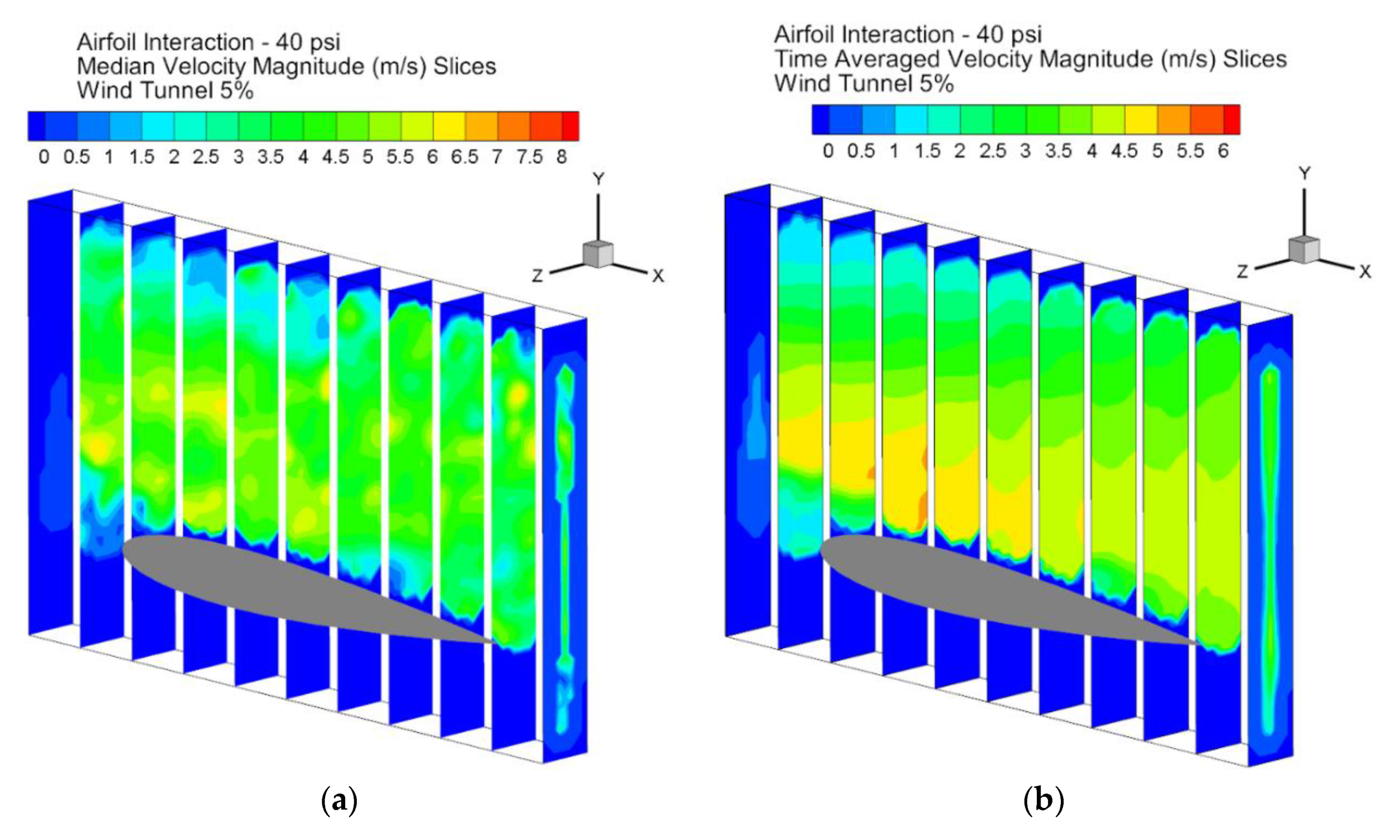
With the inclusion of the vortex tube, the presence of the vortex near the surface of the airfoil is immediately noticeable. As discussed in the review of the numerical simulations of Garmann and Visbal [5], the splitting of the vortex over the two airfoil surfaces can be observed in Figure 24.
When increasing the pressure setting of the vortex tube, the interaction is less visible due to the expansion of the generated vortex after traveling downstream. This problem is evident in the velocity maps, especially at the 40 psi setting shown in Figure 25, where the vortex has already expanded to fill much of the observed volume. Thus, in future tests, a balance must be found between avoiding the effects of the apparatus wake and maintaining the vortex further downstream. Despite the disruption of flow throughout the volume, the time-averaged velocity maps such as that of Figure 25b for the 40 psi setting indicate that the faster-moving vortex core is still reaching the leading edge of the airfoil, though its strength has been diminished during the expansion of the vortex.
3.6. 3D Airfoil Interaction Test Vorticity Data
The presence of the vortex core at the surface of the airfoil was further analyzed by calculating the x-vorticity of the flow field for each test. However, since the vortices had already dissipated and expanded considerably before reaching the observed volume, these graphs were of limited use in analyzing the vortex interaction with the airfoil. The most useful of these graphs is shown in Figure 26, which is the vorticity data for the “control” case (no vortex tube) along the case with a vortex tube set at 40 psi. The maps are left semi-translucid to allow the airfoil location be seen. Here the regions of relatively high vorticity are scattered throughout the flow field, and although one such region is present near the leading edge of the airfoil, the vorticity has already decreased so significantly that it is difficult to identify the path of the vortex core over the airfoil with this method, thus, the Q-criterion was used to obtain a better representation of the vortex interaction with the airfoil, as will be discussed in the following.
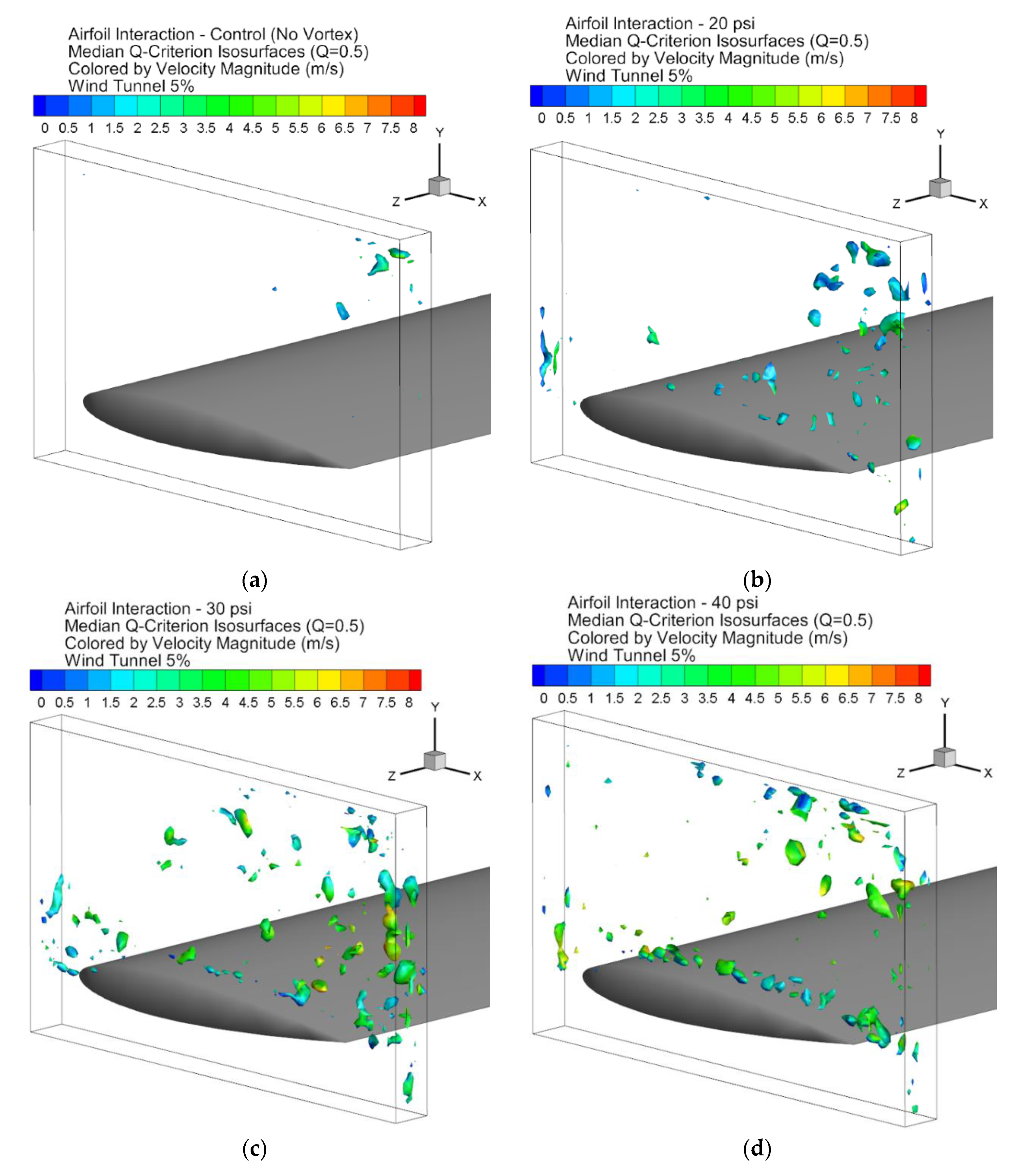
The Q-criterion was evaluated in a similar manner to the previous tomographic tests, but due to the decreased strength of the vortices, a lower value of Q = 0.5 was used when graphing the isosurfaces. Moreover, is noteworthy to mention that isosurfaces of Q = 0 present the condition of the flow after the vortices have dissipated and indicate regions in which the vorticity and strain rate are equal and, as such, these isosurfaces are located throughout the flow field due to the smaller turbulent scales and absence of high-strength large vortices [26]. As presented in Figure 27, data from the control test established that minimal vorticity was present at the surface of the airfoil in the absence of the vortex generator.
With the inclusion of the vortex generator at 20 psi, the effect of the vortex begins to take shape, but the 30 and 40 psi settings, also shown in Figure 27, more clearly illustrate the influence of the vortex on the airfoil boundary layer. Similarly, to the velocity data, the isosurfaces present upstream of the leading edge of the airfoil indicate that the vortex is being split over the airfoil and maintaining at least a part of its vorticity as it does so. This agrees with the description presented by the numerical simulation in the literature of the behavior of the incident vortex after sweeping spanwise across the airfoil [5], even though this test did not involve movement of the vortex generator.
4. Conclusions
A study of the suitability of a pressurized vortex tube for the generation of streamwise vortices was examined using state-of-the-art 2D and 3D PIV techniques and associated analysis methodology. Significant patterns and their distinctiveness occurring for the various conditions were observed. The observations from 2D analyses, while projecting features of the flows, quickly revealed limitations that were then unveiled from the 3D renderings. The complex patterns expected from a vortex tube exit flow and its interaction with a downstream airfoil using velocity and the derived properties such as streamlines, vorticity, and Q-criterion at different conditions were captured from different perspective views. It was found from these tests that increasing the air supply pressure improves the strength of the vortex at the exit of the device and allows the structures to be maintained more consistently further downstream. When the vortex velocity is greater than that of the freestream flow, a large difference in velocity between the vortex and freestream also contributed to keeping the vortex structure intact, while increasing entrainment of the freestream flow. In contrast, near the outlet, vortex strength dissipated faster with a larger difference in velocities. Low freestream velocities also reduced the degree of dissipation of the vortices after the initial reduction and allowed the vortex cores to retain their strength after traveling downstream. The relation between vorticity and travel distance was observed to be nonlinear due to significant reduction in vorticity near the outlet, followed by a more gradual decline in vortex strength.
Some limited testing on the generated streamwise vortices and a downstream airfoil produced data in agreement with the simulations from the literature that support the fact that an incident vortex on an airfoil will split over both surfaces and maintain its vorticity in doing so. However, the vortices in these tests had already lost a significant portion of their energy from traveling downstream before intersecting the airfoil, making accurate measurement more difficult than in the freestream interactions tests, and additional testing should be conducted to verify these results.
For a more thorough verification of the numerical simulations [5], additional tests should be conducted analyzing the interaction of a generated streamwise vortex and a downstream airfoil. In such tests, increasing the distance between the vortex generator and the airfoil reduces the influence of the wake from the generator apparatus on the airfoil, but also leads to the strength of the vortex being diminished as it travels and expands. A balance must be found between avoiding the effects of the apparatus wake and maintaining the vortex further downstream. Additional insight into improving vortex uniformity may also be found from an analytical investigation of the vortex tube interior.
Author Contributions
Conceptualization, J.E., design and formal analysis, B.C. and J.E., experiment and data processing, A.H.U. and B.C. All authors have read and agreed to the published version of the manuscript.
Funding
This research received no external funding.
Conflicts of Interest
The authors declare no conflict of interest.
References
- Lugt, H.J. Vortex Flow in Nature and Technology; Wiley: New York, NY, USA, 1983. [Google Scholar]
- Lissaman, P.B.S.; Shollenberger, C.A. Formation Flight of Birds. Science 1970, 168, 1003–1005. [Google Scholar] [CrossRef] [PubMed]
- Blake, W.B.; Bieniawski, S.R.; Flanzer, T.C. Surfing aircraft vortices for energy. J. Def. Model. Simul. 2015, 12, 31–39. [Google Scholar] [CrossRef]
- Syred, N.; Beér, J.M. Combustion in swirling flows: A review. Combust. Flame 1974, 23, 143–201. [Google Scholar] [CrossRef]
- Garmann, D.J.; Visbal, M.R. Interactions of a streamwise-oriented vortex with a finite wing. J. Fluid Mech. 2015, 767, 782–810. [Google Scholar] [CrossRef]
- Gavrilović, N.N.; Rašuo, B.P.; Dulikravich, G.S.; Parezanović, V.B. Commercial aircraft performance improvement using winglets. FME Trans. 2015, 43, 1–8. [Google Scholar] [CrossRef] [Green Version]
- Rostamzadeh, N.; Hansen, K.L.; Kelso, R.M.; Dally, B.B. The formation mechanism and impact of streamwise vortices on NACA 0021 airfoil's performance with undulating leading edge modification. Phys. Fluids 2014, 26, 107101. [Google Scholar] [CrossRef]
- Anderson, J.D. Fundamentals of Aerodynamics, 6th ed.; McGraw-Hill Education: New York, NY, USA, 2017. [Google Scholar]
- NASA Glenn Research Center. Downwash Effects on Lift. 2015. Available online: https://www.grc.nasa.gov/WWW/k-12/airplane/downwash.html (accessed on 10 March 2020).
- McLean, D. Wingtip Devices: What They Do and How They Do It. In Proceedings of the Boeing Performance and Flight Operations Engineering Conference, Seattle, WA, USA, 22–23 September 2005. [Google Scholar]
- Talay, T.A. Introduction to the Aerodynamics of Flight; Technical Report; NASA SP367: Washington, DC, USA, 1975.
- Whitcomb, R.T. A Design Approach and Select Wind-Tunnel Results at High Subsonic Speeds for Wing-Tip Mounted Winglets; NASA Langley Research Center: Hampton, VA, USA, 1976.
- Federal Aviation Administration. Pilot and Air Traffic Controller Guide to Wake Turbulence. Available online: https://www.faa.gov/training_testing/training/media/wake/04sec2.pdf (accessed on 10 March 2020).
- Tao, Y.; Liu, Z.; Xiong, N.; Sun, Y.; Lin, J. Optimization of Positional Parameters of Close-Formation Flight for Blended-Wing-Body Configuration. Heliyon 2018, 4, e01019. [Google Scholar]
- Mohiuddin, M.; Elbel, S. A Fresh Look At Vortex Tubes Used As Expansion Device in Vapor Compression Systems. In Proceedings of the 15th International Refrigeration and Air Conditioning Conference, West Lafayette, IN, USA, 14–17 July 2014. [Google Scholar]
- Rašuo, B. The influence of Reynolds and Mach numbers on two-dimensional wind-tunnel testing: An experience. Aeronaut. J. 2011, 115, 249–254. [Google Scholar] [CrossRef]
- Rašuo, B. Scaling between Wind Tunnels-Results Accuracy in Two-Dimensional Testing. Trans. Jpn. Soc. Aeronaut. Space Sci. 2012, 55, 109–115. [Google Scholar] [CrossRef] [Green Version]
- Damljanović, D.; Isaković, J.; Rašuo, B. T-38 wind-tunnel data quality assurance based on testing of a standard model. J. Aircr. 2013, 50, 1141–1149. [Google Scholar] [CrossRef]
- Ocokoljić, G.; Damljanović, D.; Vuković, D.; Rašuo, B.P. Contemporary Frame of Measurement and Assessment of Wind-Tunnel Flow Quality in a Low-Speed Facility. FME Trans. 2018, 46, 429–442. [Google Scholar] [CrossRef]
- Damljanović, D.; Vuković, D.; Ocokoljić, G.; Isaković, J.; Rašuo, B. A Study of Wall-Interference Effects in Wind-Tunnel Testing of a Standard Model at Transonic Speeds. In Proceedings of the 30th ICAS Congress, Daejeon, Korea, 25–30 September 2016. [Google Scholar]
- Barlow, J.B.; Rae, W.H.; Pope, A. Low Speed Wind Tunnel Testing, 3rd ed.; John Wiley&Sons, Ltd.: New York, NY, USA, 1999. [Google Scholar]
- Haque, A.U.; Asrar, W.; Omar, A.A.; Sulaeman, E.; Ali, M.J.S. Comparison of data correction methods for blockage effects in semispan wing model testing. In EPJ Web of Conferences; EFM15—Experimental Fluid Mechanics; EDP Sciences: Les Ulis, France, 2015; Volume 114, p. 02129. [Google Scholar] [CrossRef] [Green Version]
- Raffel, M.; Willert, C.E.; Scarano, F.; Kähler, C.J.; Wereley, S.T.; Kompenhans, J. Particle Image Velocimetry: A Practical Guide; Springer: Berlin/Heidelberg, Germany, 2018. [Google Scholar]
- Scarano, F. Tomographic PIV: Principles and practice. Meas. Sci. Technol. 2014, 24, 012001. [Google Scholar] [CrossRef]
- Ullah, A.H.; Fabijanic, C.; Estevadeordal, J. Advanced Measurements and Analyses of Flow Past Three-Cylinder Rotating System. In Proceedings of the AIAA2020-2671, AIAA Aviation Forum, Reno, NV, USA, 8 June 2020. [Google Scholar]
- Carlson, B.M. Generation and Analysis of Streamwise Vortices from Vortex Tube Apparatus. Master’s Thesis, North Dakota State University, Fargo, ND, USA, May 2020. [Google Scholar]
- Hunt, J.C.; Wray, A.A.; Moin, P. Eddies, Streams, and Convergence Zones in Turbulent Flows. In Proceedings of the 1988 Summer Program, Stanford, CA, USA, 31 December 1988. [Google Scholar]
- Jeong, J.; Hussain, F. On the identification of a vortex. J. Fluid Mech. 1995, 285, 69–94. [Google Scholar] [CrossRef]
- Kolář, V. Vortex identification: New requirements and limitations. Int. J. Heat Fluid Flow 2007, 28, 638–652. [Google Scholar] [CrossRef]
- Press, W.H.; Teukolsky, S.A.; Vetterling, W.T.; Flannery, B.P. Numerical Recipes, the Art of Scientific Computing, 3rd ed.; Cambridge University Press: Cambridge, UK, 2007. [Google Scholar]
- Leibovich, S.; Stewartson, K. A sufficient condition for the instability of columnar vortices. J. Fluid Mech. 1983, 126, 335–356. [Google Scholar] [CrossRef]
- Leibovich, S. The structure of vortex breakdown. Annu. Rev. Fluid Mech. 1978, 10, 221–246. [Google Scholar] [CrossRef]
- Visbal, M. Computed unsteady structure of spiral vortex breakdown on delta wings. In Proceedings of the AIAA Fluid Dynamics Conference, New Orleans, LA, USA, 17–20 June 1996. [Google Scholar]
- Drazin, P.G.; Reid, W.H. Hydrodynamic Stability, 2nd ed.; Cambridge University Press: Cambridge, UK, 2004. [Google Scholar]
- Tennekes, H.; Lumley, J.L. A First Course in Turbulence; MIT Press: Cambridge, MA, USA, 1972. [Google Scholar]
- Escudier, M.P. Observations of the flow produced in a cylindrical container by a rotating endwall. Exp. Fluids 1984, 2, 189–196. [Google Scholar] [CrossRef]
- Naumov, I.V.; Kashkarova, M.V.; Mikkelsen, R.F.; Okulov, V.L. The structure of the confined swirling flow under different phase boundary conditions at the fixed end of the cylinder. Thermophys. Aeromechanics 2020, 27, 89–94. [Google Scholar] [CrossRef]
- Sarpkaya, T. Vortex Breakdown in Swirling Conical Flows. AIAA J. 1971, 9, 1792–1799. [Google Scholar] [CrossRef]
- Hama, F.R. Streaklines in a perturbed shear flow. Phys. Fluids 1962, 5, 644–650. [Google Scholar] [CrossRef]
- Benjamin, T.B. Theory of the vortex breakdown phenomenon. J. Fluid Mech. 1962, 14, 593–629. [Google Scholar] [CrossRef]
Figure 1.
Downwash and upwash generation from wingtip vortices [11].
Figure 1.
Downwash and upwash generation from wingtip vortices [11].

Figure 2.
Schematic of vortex tube method of operation.

Figure 3.
Photography of the pressurized vortex tube and its CAD model inside the wind tunnel and in a typical configuration upstream of an airfoil. Geometry and dimensions (inches) shown.
Figure 3.
Photography of the pressurized vortex tube and its CAD model inside the wind tunnel and in a typical configuration upstream of an airfoil. Geometry and dimensions (inches) shown.

Figure 4.
Schematic of standard particle image velocimetry (PIV) (a), photography of the laser beam path (b), the tomographic four-camera arrangement (c), and the particle seeding system components (d), and schematic of the laser illumination for the vortex tube (e) and airfoil (f) data acquisition campaigns.

Figure 5.
Instantaneous 2D near region velocity map (a,c) and their streamlines (b,d) for 40 psi, 3% freestream wind tunnel setting (a,b) and for 20 psi, 20% freestream wind tunnel setting (c,d).
Figure 5.
Instantaneous 2D near region velocity map (a,c) and their streamlines (b,d) for 40 psi, 3% freestream wind tunnel setting (a,b) and for 20 psi, 20% freestream wind tunnel setting (c,d).

Figure 6.
Annular structure at vortex tube exit region instant streamlines (30 psi, 20% freestream).
Figure 6.
Annular structure at vortex tube exit region instant streamlines (30 psi, 20% freestream).

Figure 7.
Instantaneous vortex-tube flow at near region. Data at 3%, 5%, 10%, and 20% freestream wind tunnel speed settings (rows) for three different vortex tube pressures (columns).
Figure 7.
Instantaneous vortex-tube flow at near region. Data at 3%, 5%, 10%, and 20% freestream wind tunnel speed settings (rows) for three different vortex tube pressures (columns).

Figure 8.
Time-averaged vortex-tube flow at near region. Data at 3%, 5%, 10%, and 20% freestream wind tunnel speed settings (rows) for three different vortex tube pressures (columns).
Figure 8.
Time-averaged vortex-tube flow at near region. Data at 3%, 5%, 10%, and 20% freestream wind tunnel speed settings (rows) for three different vortex tube pressures (columns).

Figure 9.
Instantaneous vortex-tube flow: downstream region data at 5% (a), 10% (b), and 20% (c) wind tunnel speeds for the 40 psi vortex condition showing the 2D version of the flow that the downstream airfoil will encounter.
Figure 9.
Instantaneous vortex-tube flow: downstream region data at 5% (a), 10% (b), and 20% (c) wind tunnel speeds for the 40 psi vortex condition showing the 2D version of the flow that the downstream airfoil will encounter.

Figure 10.
Average vortex-tube flow: downstream region data at 5% (a), 10% (b), and 20% (c) wind tunnel speeds for the 40 psi vortex condition showing the 2D version of the flow that the downstream airfoil will encounter.
Figure 10.
Average vortex-tube flow: downstream region data at 5% (a), 10% (b), and 20% (c) wind tunnel speeds for the 40 psi vortex condition showing the 2D version of the flow that the downstream airfoil will encounter.

Figure 11.
Instantaneous near region vorticity map for 40 psi, 5% wind tunnel speed setting.

Figure 12.
Instantaneous velocity vector slices normal to streamwise direction compared at 3% wind tunnel setting and vortex tube pressures of 20 psi (a) and 40 psi (b), and comparing at a vortex pressure of 20 psi the freestreams from wind tunnel settings of 5% (c) and 10% (d).
Figure 12.
Instantaneous velocity vector slices normal to streamwise direction compared at 3% wind tunnel setting and vortex tube pressures of 20 psi (a) and 40 psi (b), and comparing at a vortex pressure of 20 psi the freestreams from wind tunnel settings of 5% (c) and 10% (d).

Figure 13.
Instantaneous velocity vector slices for 3% freestream and 30 psi vortex settings (a) and 20% freestream and 40 psi settings (b).
Figure 13.
Instantaneous velocity vector slices for 3% freestream and 30 psi vortex settings (a) and 20% freestream and 40 psi settings (b).

Figure 14.
Instantaneous streamlines for freestream and vortex settings of 3% and 20 psi (a), 3% and 30 psi (b), 3% and 40 psi (c), and 20% and 30 psi (d).
Figure 14.
Instantaneous streamlines for freestream and vortex settings of 3% and 20 psi (a), 3% and 30 psi (b), 3% and 40 psi (c), and 20% and 30 psi (d).

Figure 15.
Time-averaged 3D velocity vector slices for 3% freestream at 20 and 40 psi cases.

Figure 16.
Time-averaged 3D velocity vector slices for the 10% freestream and 30 psi vortex pressure case from two perspective views.
Figure 16.
Time-averaged 3D velocity vector slices for the 10% freestream and 30 psi vortex pressure case from two perspective views.

Figure 17.
Time-averaged 3D velocity vector slices for the 20% freestream and 40 psi vortex pressure case from two perspective views.
Figure 17.
Time-averaged 3D velocity vector slices for the 20% freestream and 40 psi vortex pressure case from two perspective views.

Figure 18.
Time-averaged 3D velocity vector contour maps for the stronger 40 psi vortex setting at two freestream conditions: 3% (a) and 10% (b).
Figure 18.
Time-averaged 3D velocity vector contour maps for the stronger 40 psi vortex setting at two freestream conditions: 3% (a) and 10% (b).

Figure 19.
Instantaneous vorticity slices for 40 psi and the 3% (a) and 5% (b) freestream settings.

Figure 20.
Instantaneous Q-Criterion isosurfaces for the 3% freestream setting and vortex pressure set at 30 psi (a,b) and 40 psi (c,d), each from two perspective views.
Figure 20.
Instantaneous Q-Criterion isosurfaces for the 3% freestream setting and vortex pressure set at 30 psi (a,b) and 40 psi (c,d), each from two perspective views.

Figure 21.
Vortex dissipation through tomography region for (a) 3%, (b) 5%, (c) 10%, and (d) 20% freestream wind tunnel settings.
Figure 21.
Vortex dissipation through tomography region for (a) 3%, (b) 5%, (c) 10%, and (d) 20% freestream wind tunnel settings.

Figure 22.
Vortex dissipation numerical x-derivative for (a) 3%, (b) 5%, (c) 10%, and (d) 20% freestream wind tunnel settings.
Figure 22.
Vortex dissipation numerical x-derivative for (a) 3%, (b) 5%, (c) 10%, and (d) 20% freestream wind tunnel settings.

Figure 23.
Airfoil interaction control (without the vortex tube) instantaneous median frame: (a) velocity maps and (b) velocity vector.
Figure 23.
Airfoil interaction control (without the vortex tube) instantaneous median frame: (a) velocity maps and (b) velocity vector.

Figure 24.
Airfoil interaction instantaneous median frame velocity maps with a 5% freestream setting and the vortex generator set at 20 psi (a) and 40 psi (b).
Figure 24.
Airfoil interaction instantaneous median frame velocity maps with a 5% freestream setting and the vortex generator set at 20 psi (a) and 40 psi (b).

Figure 25.
Airfoil interaction: (a) instantaneous median frame velocity maps and (b) average velocity maps; vortex generator, 40 psi.
Figure 25.
Airfoil interaction: (a) instantaneous median frame velocity maps and (b) average velocity maps; vortex generator, 40 psi.

Figure 26.
Airfoil interaction vorticity flow: instantaneous median frame of x-vorticity maps for control (no vortex tube) and vortex generator set at 40 psi; translucent view to allow airfoil view.
Figure 26.
Airfoil interaction vorticity flow: instantaneous median frame of x-vorticity maps for control (no vortex tube) and vortex generator set at 40 psi; translucent view to allow airfoil view.

Figure 27.
Airfoil interaction with q-criterion isosurfaces: control (no vortex tube) instantaneous median frame (a), and with the vortex tube set at 20 psi (b), 30 psi (c), and 40 psi (d).
Figure 27.
Airfoil interaction with q-criterion isosurfaces: control (no vortex tube) instantaneous median frame (a), and with the vortex tube set at 20 psi (b), 30 psi (c), and 40 psi (d).


Table 1.
Experimental conditions.
| WT Set (%) | WT Vel (m/s) | VT (psi) | VT Exit Plane Vel (m/s) | Uo (m/s) (V_avg) | Re (Uo × d/ν) | ||
|---|---|---|---|---|---|---|---|
| Vx_avg | Vy_avg | Vz_avg | |||||
| 3 | 0.21 | 0.21 | 1.01 | 1.07 | 5.77 | 6.95 | 2982 |
| 3 | 0.21 | 0.21 | 1.56 | 1.79 | 9.65 | 11.07 | 4752 |
| 3 | 0.21 | 0.21 | 2.71 | -2.19 | 9.16 | 11.88 | 5099 |
| 5 | 2.9 | 2.9 | 2.58 | 1.24 | 5.37 | 6.66 | 2856 |
| 5 | 2.9 | 2.9 | 2.38 | 1.82 | 6.90 | 7.51 | 3222 |
| 5 | 2.9 | 2.9 | 2.46 | -1.40 | 7.23 | 9.24 | 3965 |
| 10 | 4.32 | 4.32 | 3.20 | 1.09 | 6.49 | 7.08 | 3039 |
| 10 | 4.32 | 4.32 | 3.44 | 1.23 | 6.20 | 7.31 | 3135 |
| 10 | 4.32 | 4.32 | 3.69 | 1.60 | 6.91 | 8.96 | 3843 |
| 20 | 8.58 | 8.58 | 6.73 | 1.03 | 2.74 | 7.17 | 3077 |
| 20 | 8.58 | 8.58 | 5.83 | 1.45 | 3.82 | 8.12 | 3483 |
| 20 | 8.58 | 8.58 | 6.48 | 1.12 | 3.52 | 9.85 | 4225 |
Table 2.
Maximum time-averaged vorticity measurements at the vortex generator outlet.
| Ω (1/s) | 3% | 5% | 10% | 20% |
|---|---|---|---|---|
| 20 psi | 1695.210 | 1379.880 | 2368.070 | 1325.320 |
| 30 psi | 3470.530 | 2523.750 | 2152.670 | 1354.960 |
| 40 psi | 3239.890 | 2524.980 | 2479.220 | 1794.040 |
Table 3.
Maximum time-averaged vorticity measurements at maximum x-value.
| Ω (1/s) | 3% | 5% | 10% | 20% |
|---|---|---|---|---|
| 20 psi | 739.689 | 623.144 | 624.112 | 593.548 |
| 30 psi | 696.067 | 653.810 | 588.809 | 617.909 |
| 40 psi | 984.326 | 1012.160 | 808.438 | 926.641 |
© 2020 by the authors. Licensee MDPI, Basel, Switzerland. This article is an open access article distributed under the terms and conditions of the Creative Commons Attribution (CC BY) license (http://creativecommons.org/licenses/by/4.0/).
Share and Cite
MDPI and ACS Style
Carlson, B.; Ullah, A.H.; Estevadeordal, J. Experimental Investigation of Vortex-Tube Streamwise-Vorticity Characteristics and Interaction Effects with a Finite-Aspect-Ratio Wing. Fluids 2020, 5, 122. https://doi.org/10.3390/fluids5030122
AMA Style
Carlson B, Ullah AH, Estevadeordal J. Experimental Investigation of Vortex-Tube Streamwise-Vorticity Characteristics and Interaction Effects with a Finite-Aspect-Ratio Wing. Fluids. 2020; 5(3):122. https://doi.org/10.3390/fluids5030122
Chicago/Turabian StyleCarlson, Bailey, Al Habib Ullah, and Jordi Estevadeordal. 2020. "Experimental Investigation of Vortex-Tube Streamwise-Vorticity Characteristics and Interaction Effects with a Finite-Aspect-Ratio Wing" Fluids 5, no. 3: 122. https://doi.org/10.3390/fluids5030122