Forecasting wildfires in major forest types of India
 Manish P. Kale1*†
  Asima Mishra1† Satish Pardeshi1† Suddhasheel Ghosh2‡ D. S. Pai3‡ Parth Sarathi Roy4,§
- 1Centre for Development of Advanced Computing (C-DAC), Pune, India
- 2Faculty of Engineering and Technology, MGM University, Aurangabad, India
- 3Institute of Climate Change Studies (ICCS), Kottayam, India
- 4World Resources Institute, New Delhi, India
Severity of wildfires witnessed in different parts of the world in the recent times has posed a significant challenge to fire control authorities. Even when the different fire early warning systems have been developed to provide the quickest warnings about the possible wildfire location, severity, and danger, often it is difficult to deploy the resources quickly to contain the wildfire at a short notice. Response time is further delayed when the terrain is complex. Early warning systems based on physics-based models, such as WRF-FIRE/SFIRE, are computationally intensive and require high performance computing resources and significant data related to fuel properties and climate to generate forecasts at short intervals of time (i.e., hourly basis). It is therefore that when the objective is to develop monthly and yearly forecasts, time series models seem to be useful as they require lesser computation power and limited data (as compared to physics-based models). Long duration forecasts are useful in preparing an efficient fire management plan for optimal deployment of resources in the event of forest fire. The present research is aimed at forecasting the number of fires in different forest types of India on a monthly basis using “Autoregressive Integrated Moving Average” time series models (both univariate and with regressors) at 25 km × 25 km spatial resolution (grid) and developing the fire susceptibility maps using Geographical Information System. The performance of models was validated based on the autocorrelation function (ACF), partial ACF, cumulative periodogram, and Portmanteau (L-Jung Box) test. Both the univariate- and regressor-based models performed equally well; however, the univariate model was preferred due to parsimony. The R software package was used to run and test the model. The forecasted active fire counts were tested against the original 3 years monthly forecasts from 2015 to 2017. The variation in coefficient of determination from 0.94 (for year 1 forecast) to 0.64 (when all the 3-year forecasts were considered together) was observed for tropical dry deciduous forests. These values varied from 0.98 to 0.89 for tropical moist deciduous forest and from 0.97 to 0.88 for the tropical evergreen forests. The forecasted active fire counts were used to estimate the future forest fire frequency ratio, which has been used as an indicator of forest fire susceptibility.
Introduction
Numerous studies have revealed that forest fires have become increasingly severe (Reilly et al., 2017; Singleton et al., 2019). Several incidences of catastrophic wildfires have been reported in the last 4–5 years for example in California, USA (Du et al., 2019) and Australia (Bowman et al., 2020). In the Indian context, an unprecedented wildfire occurred in the state of Uttarakhand in 2016 (Sati and Juyal, 2016), which burnt 2,166 km2 within and outside the forest area (Jha et al., 2016). As the forests are habitats for the tribal/natural forest dwellers and the storehouse of floral and faunal biodiversity, it is important to safeguard them from a devastating wildfire. It is difficult and costly to contain the wildfire after it has spread significantly, thus mid- to long-duration forecasts (monthly and yearly) of the potential forest fires are important to develop well-informed mitigation strategies.
Some of the previous studies were carried out to forecast the number of forest fires using the ARIMA (Autoregressive Integrated Moving Average) model (Slavia et al., 2019; Kadir et al., 2020); estimate the probability of fire on a defined day using Probit model (Albertson et al., 2009); model the number of forest fires using longitudinal negative bionomial (NB) and zero-inflated negative bionomial (ZNIB) mixed models (Viedma et al., 2018); predict fire activity for 1–5 days in the future using MODIS satellite data active fire count and ERA-interim reanalysis-based weather data using Poisson’s regression method (Graff et al., 2020); and map the fire risk using machine learning and satellite vegetation index time series (Michael et al., 2021) and an analytical hierarchical process (Sivrikaya and Kucuk, 2021).
The impact of different drivers on the occurrence of forest fires has also been studied in numerous studies (Westerling et al., 2002; Rodrigues et al., 2014; Biswas et al., 2015; Kale et al., 2017; Viedma et al., 2018). Extreme climate events, i.e., ENSO (El Niño Southern Oscillation), NAO (North Atlantic Oscillation), and AMO (Atlantic Multi-decadal Oscillation) are found to be associated with forest fires (Siegert and Hoffmann, 2000; Siegert et al., 2001; Patra et al., 2005; Kidzberger et al., 2007; N’Datchoh et al., 2015; Devischer et al., 2016). Kale et al. (2017) found an interrelation of NINO 3 index with a number of forest fires in India. The drivers such as fuel type (Bond and Keeley, 2005), population/human influence (Bowman et al., 2011), topography (Rollins et al., 2002), distance to settlement and roads (Laurance et al., 2009), aspect (Allexander et al., 2006), rainfall, and temperature (McKenzie et al., 2004; Aldersley et al., 2011) have been identified to be related to forest fires. Urbieta et al. (2019) emphasized that, despite the increasing fire risk factors, fire can be controlled and reduced provided fire suppression resources (mainly aerial) are increased. This emphasizes the need to develop integrated early warning and response systems.
Efforts have been made world-over to develop fire danger rating systems/alert systems/information systems to disseminate timely information about potential fire danger to different stakeholders. The national fire danger rating system (NFDRS) of the United States of America uses fuel type, topography, and weather as inputs to estimate fire danger for next 24 h (USDA, 2022). The Canadian Forest Fire Weather Index (FWI) system provides maps of fire danger and fire weather indices on a daily basis (Natural Resource Canada, 2022). The European Forest Fire Information System (EFFIS) provides services related to wildland fire in Europe. EFFIS provides “fire danger” forecast upto 9 days in the European region (EFFIS, 2022). Forest Survey of India uses satellite data [SNPP (Suomi-National Polar-orbiting Partnership)-VIIRS] to identify and track large forest fires on a near real-time basis in India (FSI, 2022). In addition, the sophisticated numerical two-way coupled models such as WRF-FIRE have been developed and tested for operational fire spread simulation in different countries, i.e., Israel (Mandel et al., 2014), Greece (Giannaros et al., 2020), and USA (UCAR, 2022) to quickly (hourly basis) predict the wildfire spread once the ignition location is detected.
Even when the different fire early warning systems are available to provide the quickest possible warnings about the wildfire location, severity, and danger, often, it is difficult to deploy the resources quickly to contain the wildfire at short notice. Response time is further delayed when the terrain is complex. It is therefore the mid- to long-term (monthly and yearly) fire forecasts that are the key for pre-allocating resources at potentially vulnerable locations during the fire season, hence shortening the response time of the forest fire fighting authorities.
Time series analysis (TSA) of the forest fire is useful in forecasting fire events at specified time intervals. Forecasts may be based on multiple independent (causal) variables or simply on the fire time series itself (univariate). Fire forecasts considering independent variables are based on dynamic interrelationships of wildfires and associated independent variables with respect to time. Univariate and multivariate times series models have been tested and compared previously in numerous cross-disciplinary studies, for example, for estimating tourist demand (Preez and Witt, 2003) and forecasting the medical emergency department demand (Jones et al., 2009; Sarfo et al., 2015). Some studies have found the multivariate time series models superior to univariate models (Jones et al., 2009; Sarfo et al., 2015), whereas, others have recommended univariate models over the multivariate models, for example, Iwok and Okpe (2016), recommended univariate model while studying different time series variables from Nigeria’s gross domestic products. Sethi and Mittal (2020) found the univariate ARIMA model superior to the multivariate vector autoregression model (VAR) for the prediction of air quality index. TSA is a data-intensive process and requires several years of data to derive meaningful interpretations. As compared to multivariate model, the univariate model is less data demanding.
Modern remote sensing platforms (along with ground sensor networks) have made it possible to obtain such datasets at higher temporal and spatial resolutions. For example, NASA’S Fire Information for Resource Management System distributes fire point data on daily basis within 3 h of observations by MODIS and VIIRS satellite sensors at 1 km and 375 m spatial resolution, respectively (EARTHDATA, 2022). Similarly, the network of different ground meteorological stations world over has made it possible to obtain the high-frequency data, for example, of rainfall and temperature.
There are different methods in vogue that use the time series data for forecasting. For example, linear and multiple regressions, exponential smoothing, autoregressive Integrated moving average (ARIMA), logistic regression, and Probit models have been frequently used in carrying out fire predictions (Contreras et al., 2003; Preez and Witt, 2003; Preisler and Westerling, 2007; Prestemon et al., 2012; Briët et al., 2013; Huesca et al., 2014; Zhang et al., 2016; Lei, 2017; Ye et al., 2017; Feng and Shi, 2018; Santana et al., 2018; Slavia et al., 2019). The TSA involves analysis of data collected over a specified time interval, i.e., day, month, week, or year and is useful in near future forecasting. Among different time series forecasting models, the ARIMA model has been used extensively in cross-disciplinary domains (Mujumdar and Kumar, 1990; Wangdi et al., 2010; Sarfo et al., 2015; Zhou et al., 2018; Jesus et al., 2022).
The forecasts obtained through TSA models depends upon how the variables are defined. In the present research the “active fire counts” has been used as a dependent variable, thus, the forecast is “active fire count.” The active fire count data is useful in estimating fire susceptibility using the frequency ratio method (Lee and Pradhan, 2007; Pradhan, 2010; Biswas et al., 2015; Kale et al., 2017).
The present research is aimed at (i) forecasting active forest fire counts using the ARIMA model (univariate ARIMA and ARIMA model with regressors) in prominent forests of India and (ii) deriving probabilistic fire susceptibility map in GIS using fire frequency ratio (FFR) method.
Study area
The study has been carried out in Tropical Evergreen forests (TEGF), Tropical Moist Deciduous forests (TMDF), and Tropical Dry Deciduous forests (TDDF) located in different biogeographic zones of India (Figure 1). The Indian region can be divided into ten bio-geographic zones, i.e., Trans-Himalaya, Himalaya, Desert, Semi-Arid, Western Ghats, Deccan Peninsula, Gangetic Plain, Coasts, North-East, and the Islands (Rodgers and Panwar, 1988). High elevation regions of the Himalayas receive significant snowfall. Parts of western and central regions receive meager rainfall, whereas, eastern India is one of the highest monsoon rainfall regions of the world. The type of the forest is attributed mainly to climate, soil, and past treatment (Champion and Seth, 2005). The TEGF, TDDF, and TMDF are distributed in different proportions in the Western Ghats, Deccan Peninsula, Gangetic Plain, Himalaya, and North-East regions. The temperature and precipitation in these forests vary between 8 and 38°C and 400 and 7,000 mm, respectively (Roy et al., 2015).
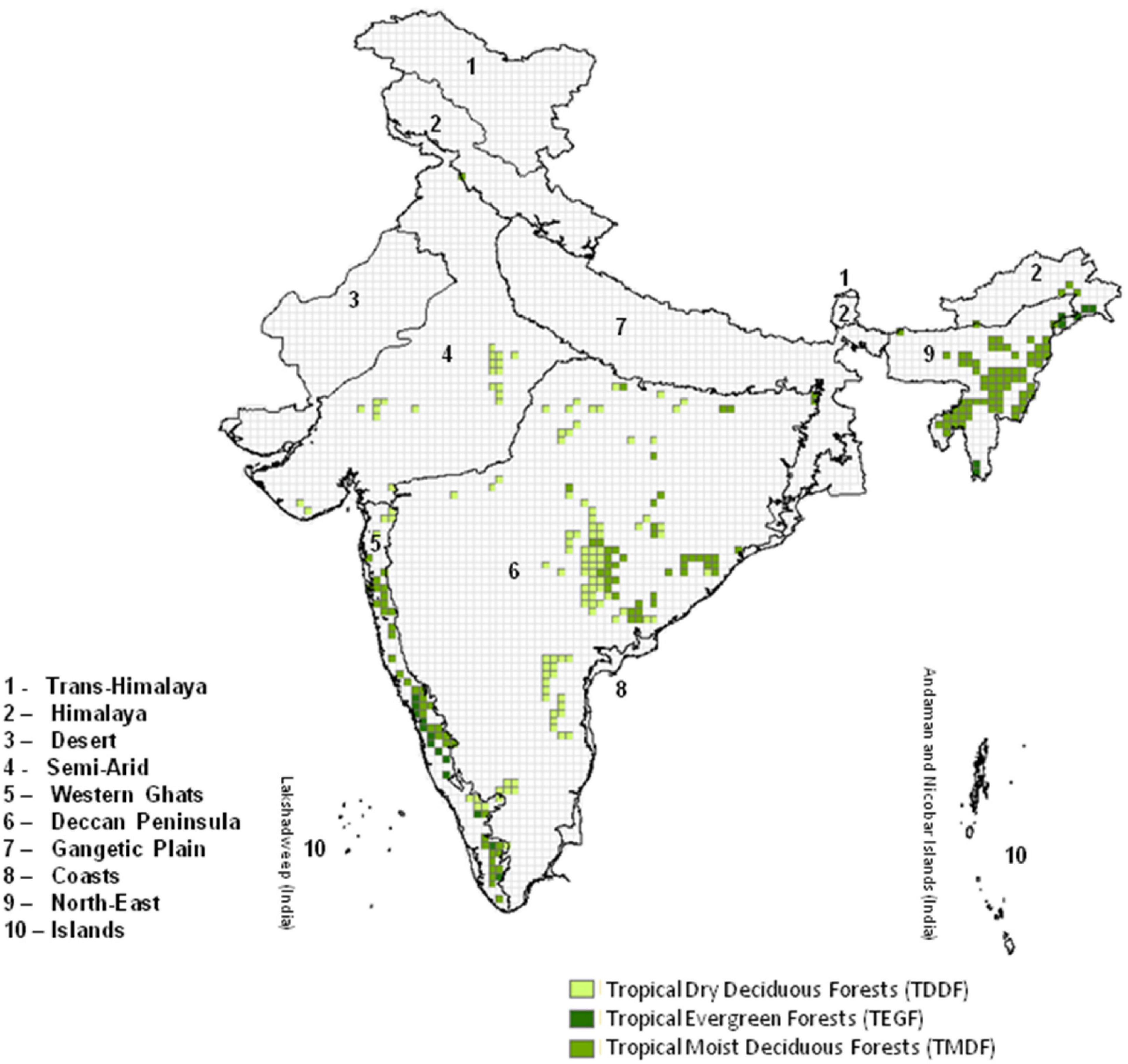
Figure 1. Study area showing different forest types (25 km grid) overlaid on the Biogeographic zones of India (Rodgers and Panwar, 1988; Rodgers et al., 2000).
The fires in TMDF are generally sporadic and patchy (Kodandpani et al., 2008). These forests become prone to fire when disturbed. Once disturbed and fragmented, the grasses become prevalent which makes these forests susceptible to fire (Woods, 1989; Suresh et al., 1996; Freifelder et al., 1998; Kodandpani et al., 2008). Fire leads to a further spread of grasses which becomes heavy and continuous, particularly where there is an open canopy (Champion and Seth, 2005). The TMDF supports significant biodiversity as they are comparatively denser and moister than TDDF. It is therefore extremely important to understand the possible future trends of forest fires in these critical forests so as to take mitigative measures. TDDF are significantly burning forests of India. These forests have associated grasses (particularly in central India) and exhibit seasonality. Leaves are shed in specific seasons, which usually start with the onset of summers. During extreme climate, due to increased temperature and dryness, significant burning happens in these forests. TEGF are comparatively lesser burnt forests due to the availability of moisture even during the fire season. These forests are confined to narrow strips in Western Ghats, North-East India, and Andaman and Nicobar Islands (Roy et al., 2015).
Forest fire generally follows a well-defined timeline in India. The fire season in India is mostly from February to June (Satendra and Kaushik, 2014; Kale et al., 2017). Every year wildfire peaks in the month of March/April and then decline at the start of the rainy season (June). Such seasonality continues year after year. However, geographical differences in the duration and peak of the season do exist, requiring in-depth analyses such as the one presented here.
Materials and methods
Different datasets were used in this research for forecasting the active forest fire counts [using univariate ARIMA model and ARIMA model with regressors (NAU, 2020)] and estimating FFR.
The dependent variable, i.e., active fire locations (2003–2017) was sourced from MODIS level 6 active fire product (MODIS, 2022). This depicted fires burning in 1 km pixel at the time of satellite overpass. Independent variables, i.e., monthly dry days (days without rainfall) and maximum average monthly temperature were estimated based on the daily rainfall grid (25 km × 25 km) and temperature grid (1° × 1°) from 2003 to 2017 obtained from India Meteorological Department (IMD; Srivastava et al., 2009; Pai et al., 2014).
Other datasets, i.e., the vegetation type map of India (scale 1:50,000) providing details of natural and semi-natural land-use and land-cover systems and the natural vegetation (Roy et al., 2015) were used to extract the TDDF, TMDF, and TEGF of India; elevation (90 m resolution) was sourced from SRTM1 and used to derive the slope map. These datasets were used as inputs for FFR estimation in addition to temperature and dry days. Biogeographic zones of India (Rodgers and Panwar, 1988; Rodgers et al., 2000) were used for zone-wise segregation of active fire and FFR.
R software package was used to run the ARIMA model (primary modules used were Forecast (Hyndman and Khandakar, 2008; Hyndman et al., 2022) and TSPred (Salles and Ogasawara, 2022). Different online resources in relation to TSA were also referred (Hyndman, 2022b; STACKOVERFLOW, 2022).
All the datasets were resampled to 25 km × 25 km grid in GIS. The forest types, i.e., TMDF, TDDF, and TEGF were extracted from the vegetation type map based on the majority class occurring in each grid. The active fire counts were extracted for each forest type on monthly basis for all the grids and all the years. The average number of dry days and maximum average temperature were extracted for TDDF, TMDF, and TEGF on a monthly basis for all the years at grid level. The geographic coordinate system and WGS 84 datum were used in the present research.
The daily rainfall and maximum average temperature data had gaps, i.e., non-availability of data for particular days or a particular month for a specified grid. These gaps were filled either by taking the average of previous and next day observations or by taking the average of two neighboring grids belonging to the same forest type and terrain conditions. Such gaps, however, were not significant and hence filling them did not affect the overall trend.
The forest type-wise monthly active fire counts, the total number of dry days, and the maximum average temperature were used as inputs to forecast the active fire counts. We avoided 0 fire counts in the model and replaced all 0 values with 1. For TDDF and TMDF and TEGF 2%, and 1% of all the observations had “no fire” incidence (0 fire counts), respectively. Further, this occurred only during the rainy season. For TEGF 3%, no fire incidences occurred during the fire season, and this was because these forests were comparatively wetter during the fire season than other forest types.
Forecasting using ARIMA model is based on the premise that the time series data is stationary, i.e., it has no trend and seasonality. The ARIMA model has three components, i.e., “AR,” “I,” and “MA.”. The “AR” or autoregression component provides information about regression of time series data with itself in different time lags. It gives clues about how significantly the data is auto-correlated, and thus the impact of past data on future forecasting could be understood (Jones et al., 2009). The “AR” analysis is also helpful in understanding whether the data is seasonal. For seasonal time series, the “AR” exhibits sinusoidal patterns. For non-stationary data, significant autocorrelation is observed even for the larger time lags, whereas, for stationary time series, autocorrelation dies down-within the initial few time lags (Mujumdar, 2022).
The “I” or integrated term provide information about how many “difference” terms are required to make the data stationary in case the time series data is non-stationary. The “difference” terms mean the difference between the current time and the past time for all the time lags.
The “MA” provides information about the number of “moving average” terms to be used. The “MA” is the average of the fixed set of previous time-period values when it is moved throughout the data sets to obtain a new time series. The “MA” can be carried out multiple times, i.e., the output of the first “MA” can again be subjected to a second “MA” and so on, till stationarity is achieved (Mujumdar, 2022).
The model belonging to ARMA family may be written as follows (Mujumdar and Kumar, 1990).
where Y(t) (t = 1, 2,….) is the time series used in the modeling; m1 is the number of AR terms; ϕj is the jth AR parameter; m2 is the number of MA terms; θj is the jth MA parameter; C is a constant; and w (t) (t = 1,2,…..) is the residual series.
Kashyap and Rao (1976) argued that time series differencing, which is an essential component of ARIMA, causes the variance to increase continuously, and hence such models cannot be used for data simulation. They may, however, be used for one-step ahead forecasting.
Identification of optimum “AR,” “I,” and “MA” terms is important to achieve stationarity. This process is time-consuming and at times may not converge for a higher denomination of “AR,” “I,” and “MA” terms, thus we used the Hyndman and Khandakar (2008) algorithm for automatic identification of these terms and avoided manual iterations. Further Hyndman and Khandakar (2008) believed that it was better to make as few differences as possible to avoid widening of the prediction intervals. Thus, they preferred the unit root test for defining the difference terms over minimizing the AICc (Corrected Akaike’s Information Criterion), which tends to lead to over differencing. AIC has, however, been used to select the orders of the AR and MA components in auto.arima model (Hyndman, 2022a). In this context, the concerns of Kashyap and Rao (1976) seem to have been addressed. The forecast module of “R” open-source package developed by Hyndman et al. (2022) was used to forecast the active fire counts.
Model calibration
The monthly forest type-wise time series data (2003–2017) were divided into two parts, i.e., “train data” (2003–2014) and “test data” (2015–2017). The “train data” was used for ARIMA model building, whereas, the “test data” was used to test the model performance (Walters, 2022).
The autocorrelation function (ACF) and partial autocorrelation function (PACF) of “train data” were plotted to investigate the “seasonality,” whereas, the cumulative periodogram was plotted to investigate the “periodicity” present in the time series. The ACF and PACF are the plots of time lags against autocorrelation values, whereas, periodogram analysis was carried out in the frequency domain and plotted between frequency and periodicity.
The Hyndman and Khandakar (2008) algorithm helped in automatically determining the number of “AR,” “I,” and “MA” terms for non-seasonal, i.e., p (AR), d (I), and q (MA) as well as seasonal components, i.e., P (AR), D (I), and Q (MA) of the data. The number of difference terms (d, where d is 0 ≤ d ≤ 2) were determined by repeated Kwiatkowski-Phillips-Schmidt-Shin (KPSS) test to achieve the “stationarity.” The algorithm does not search for every possible combination of different ARIMA terms, rather it uses a step-wise search to traverse through the model space. All the results were validated to confirm that the model residuals were white noise (significant autocorrelation was absent).
In the univariate model, only the monthly fire data from 2003 to 2017 were considered, whereas, in model with regressors, temperature and dry days (2003–2017) were also considered for forecasting forest active fire counts [in the Indian context dry days and temperature are important forest fire drivers (Kale et al., 2017)].
We used “xreg” argument under auto-arima function in R to consider regression errors for forecasting (Hyndman and Athanasopoulos, 2018). The overall functioning of ARIMA model with regressors is more or less same as the standard regression process.
Model validation
The best ARIMA model obtained was subjected to validation. This was achieved by observing the significant level of residuals of ARIMA model through plotting ACF, PACF, and cumulative periodogram, and by conducting the Portmanteau test (L-Jung Box test) (Box and Pierce, 1970; Ljung and Box, 1978; Harvey, 1993; Coghlan, 2018; Hyndman and Athanasopoulos, 2018). The insignificant ACF, PACF, and cumulative periodograms were desired for valid forecasts. The Portmanteau test was conducted based on the number of lags as suggested by Hyndman and Athanasopoulos (2018). Since data had seasonal components, the number of lags was equal to 2 m, where m is the period of seasonality [12 (monthly) in the present research]. The hypothesis was tested by analyzing p-values. The higher p-values (>0.05) depicted that the residuals were not distinguishable from white noise series, i.e., there was no serial correlation present (Hyndman and Athanasopoulos, 2018).
Post model validation, forest fires were forecasted for the year 2015 onward. The original (test data) vs. forecasted monthly fire were compared for the years 2015–2017 (36 values) by plotting them within the confidence bands of 80 and 95% level significance.
To estimate the forecasted fire at the grid level (to be used for FFR estimation), the percent monthly contribution of each grid of a particular forest type toward fire occurrence was averaged for 15 years (2003–2017) and the forecasted fire (for the year 2017) were segregated in the grids in proportion to their average percentage contribution of fire.
The FFR investigation for the year 2017 was carried out by taking different gridded themes into consideration. These included (maximum average monthly temperature, average number of dry days, monthly average of 15 years, i.e., 2003–2017), elevation, slope, and vegetation type (Figure 2).
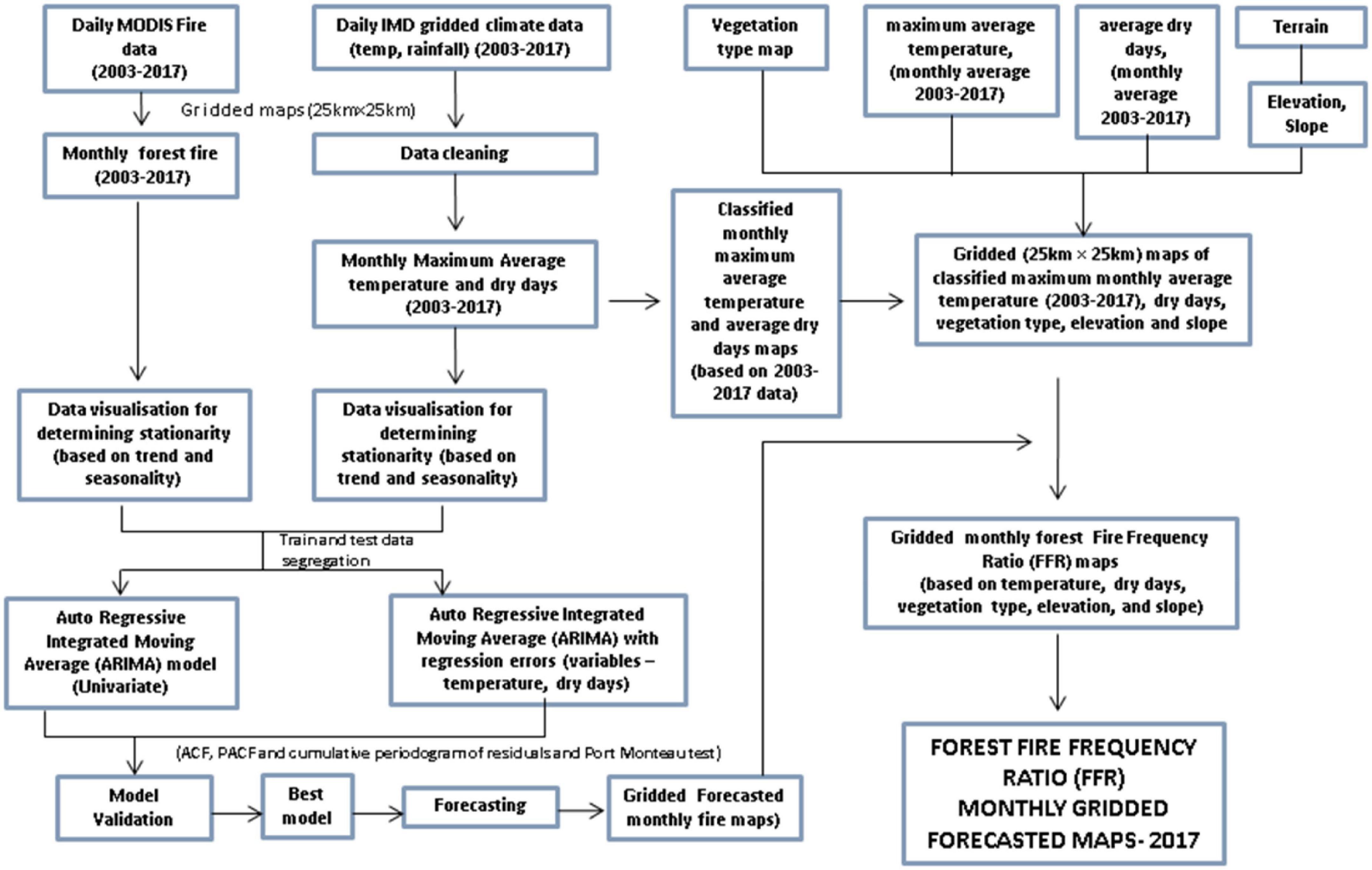
Figure 2. Methodology.
The temperature, dry days, elevation, and slope grids were classified into 5 classes, i.e., 1. Low 2. Moderate 3. High 4. Higher, and 5. Highest based on the “Jenk’s natural breaks” in GIS. The theme-wise frequency ratio was estimated by taking the ratio of “fire ratio” and “grid ratio” (Lee and Pradhan, 2007; Pradhan, 2010; Biswas et al., 2015). The “fire ratio” is the ratio of fire that occurred in a particular class of a theme (for example, fire occurred in low elevation class in “elevation” theme) and the total number of fires that occurred in that particular theme (for example total fire occurred in the elevation theme). The “grid ratio” is the ratio of the total number of grids present in a particular class of a theme to the total number of grids present in that theme. The grid-wise FFR for each theme was integrated to estimate the final grid-wise FFR (Supplementary material 1), which depicted the fire susceptibility. The higher FFR depicts higher susceptibility toward forest fire.
The forecasted FFR (2017) was compared with the original FFR (2017) to understand the variations.
Results
Forest fire incidences
The TDDF, TMDF, and TEGF depicted almost similar patterns of fire occurrences during different months of the year. Fire incidences reached the peak during summers and the trough during rainy seasons. This pattern was repeated year after year (Figure 3). The forests achieved peak fire during March/April for all the studied years. No increasing fire trend was, however, observed for any of the studied forest types. The highest incidences of fire were observed in TMDF followed by TDDF. TMDF are prominent in the North-East regions of India, where shifting cultivation is prevalent in pockets, thus the anthropogenic fire incidences are rampant. The TDDF are prominent in the Deccan Peninsula and the semi-arid regions of India which are warmer and thus the fire incidences are high, particularly during extreme climate events. The TEGF had comparatively lesser fire events as forest floors were not as dry as TDDF and TMDF.
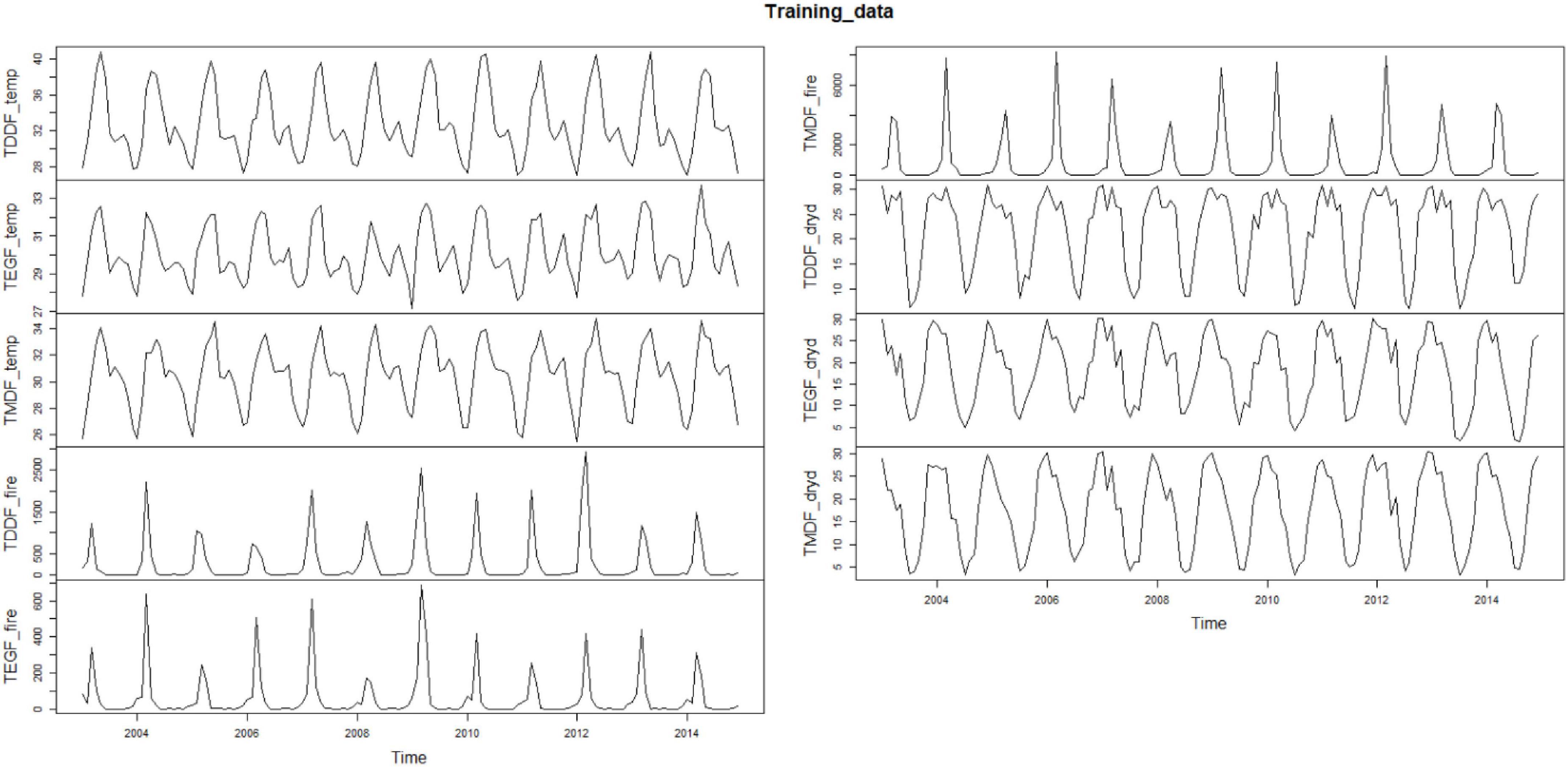
Figure 3. Training datasets—TDDF_temp, TDDF_fire, and TDDF_dryd depicts monthly average maximum temperature, monthly fire counts, and number of dry days for Tropical Dry Deciduous Forests; TMDF_temp, TMDF_fire, and TMDF_dryd depicts monthly average maximum temperature, monthly fire counts and number of dry days for Tropical Moist Deciduous Forests; TEGF_temp, TEGF_fire, and TEGF_dryd depicts monthly average maximum temperature, monthly fire counts, and number of dry days for Tropical Evergreen Forests.
The maximum average temperature had significant seasonality with not much variation in patterns for TDDF and TMDF, whereas, fluctuations were observed in TEGF, particularly in the year 2009, when the temperature reached minimum among all the studied years (Figure 3). The number of dry days was maximum in TDDF, whereas, the range of dry days was smaller for TEGF as compared to TDDF and TMDF (Figure 3).
The ACF of forest fires exhibited a gradual decay, which indicated higher autocorrelation among the subsequent lags rather than the lags at the distal end of the time series. The ACF had a sinusoidal pattern which depicted seasonality. Significant autocorrelation (both positive and negative) was present even upto the time lag of 100, which is suggestive of strong seasonality (Figure 4). Clear PACF peaks were observed in TDDF, TMDF, and TEGF (Figure 4). This is suggestive of the number of AR terms that may be required in the ARIMA model. All the forests had significant periodicities, which were reflected in the cumulative periodogram plots (Figure 4). On many instances, the periodicities crossed the limit of the significance range, which was at 95% level. Periodicities in the data were subjected to spectral analysis in the frequency domain rather than the time domain. The “cumulative periodogram” depicted the presence of significant periodicities in all the forest types.
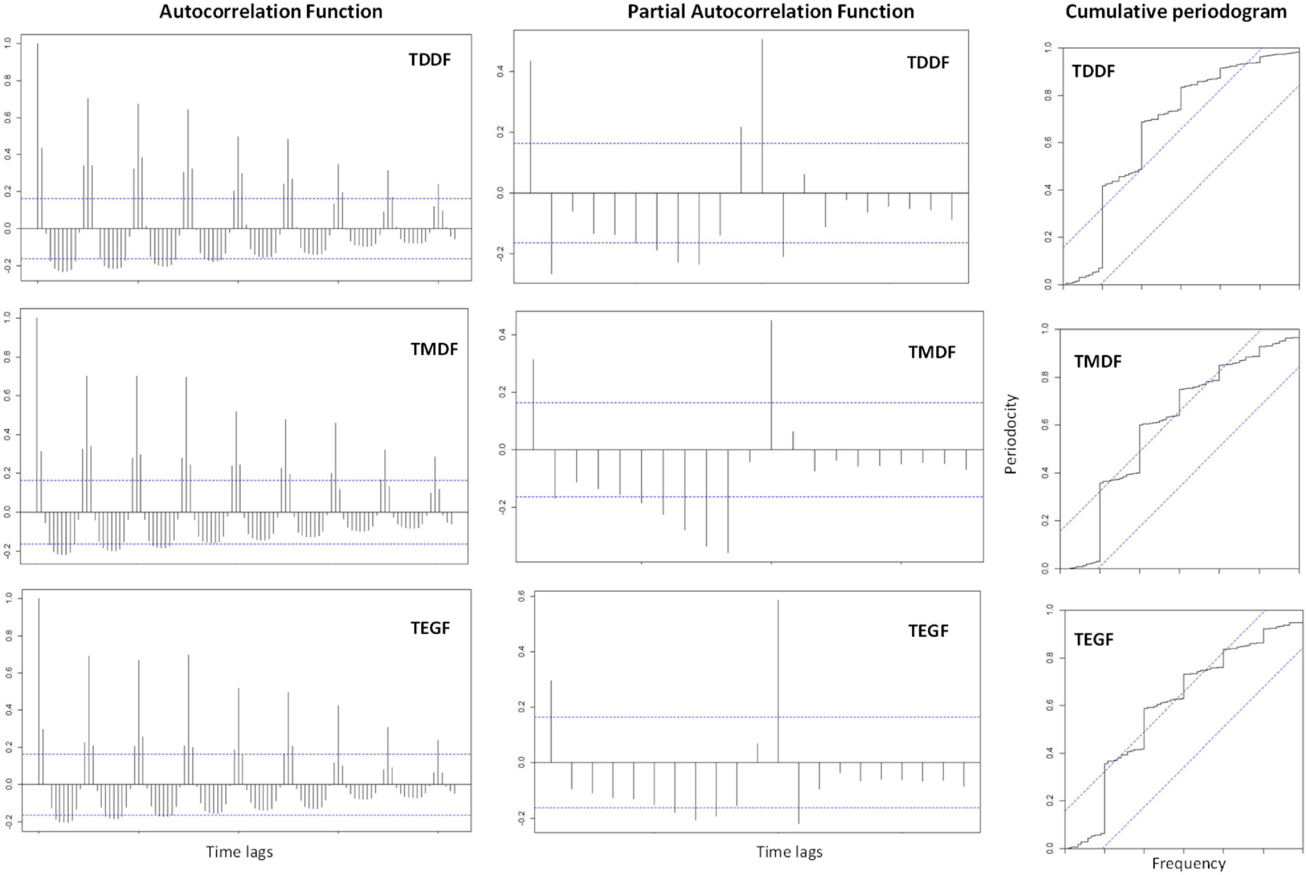
Figure 4. Autocorrelation function and partial autocorrelation function (100 lags) and cumulative Periodogram for Tropical Dry Deciduous Forests (TDDF), Tropical Moist Deciduous Forests (TMDF), and Tropical Evergreen Forests (TEGF).
Autoregressive integrated moving average models and their intercomparison
A univariate ARIMA model for TDDF, TMDF, and TEGF was developed using auto.arima function. The best model obtained using Hyndman-Khandakar algorithm had p,d,q, and P,D,Q-values of 0,0,1, and 2,1,0 for TDDF; 0,0,1, and 2,1,1 for TMDF and 1,0,0 and 2,1,2 for TEGF, respectively (Table 1 and Supplementary material 2). After applying the model, the residuals had insignificant autocorrelation and partial autocorrelation for most of the time lags for all the forest types (Figure 5). The cumulative periodogram also depicted insignificant periodicities (Figure 5).
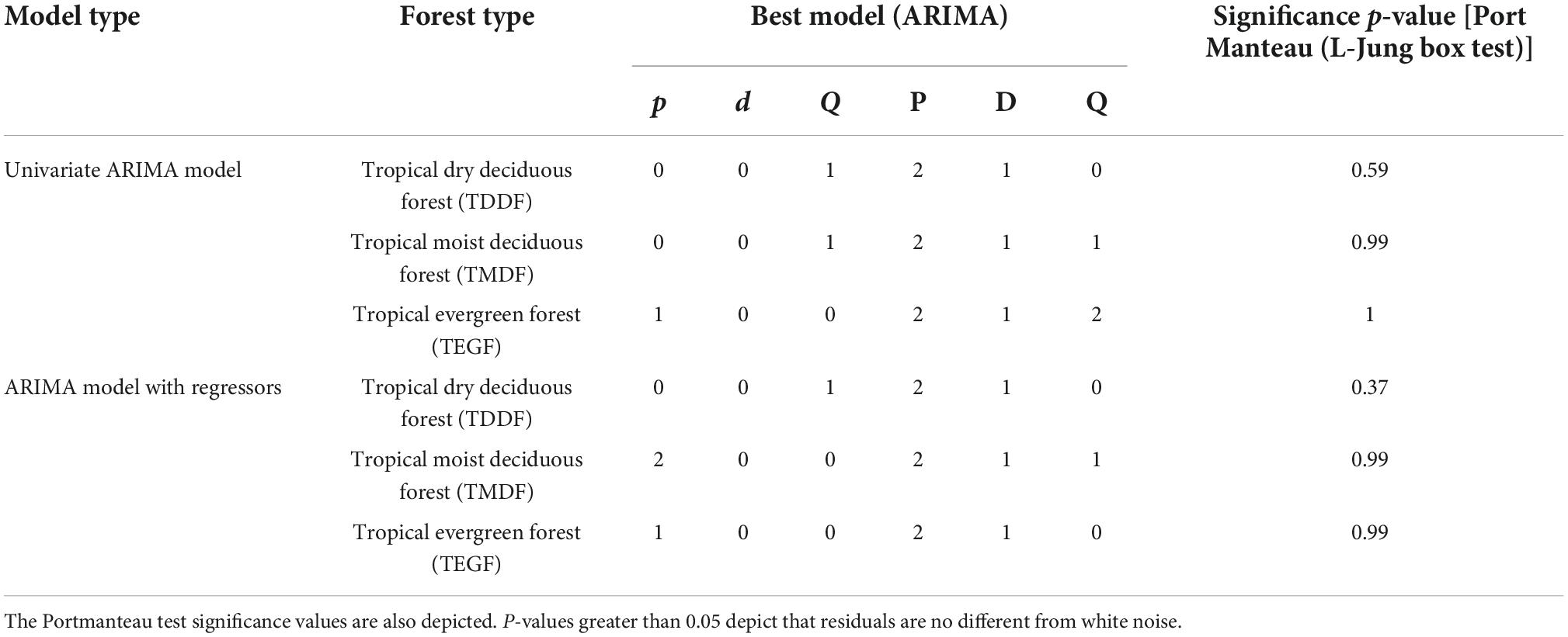
Table 1. Comparison of model results obtained through univariate ARIMA model and ARIMA model with regressors.
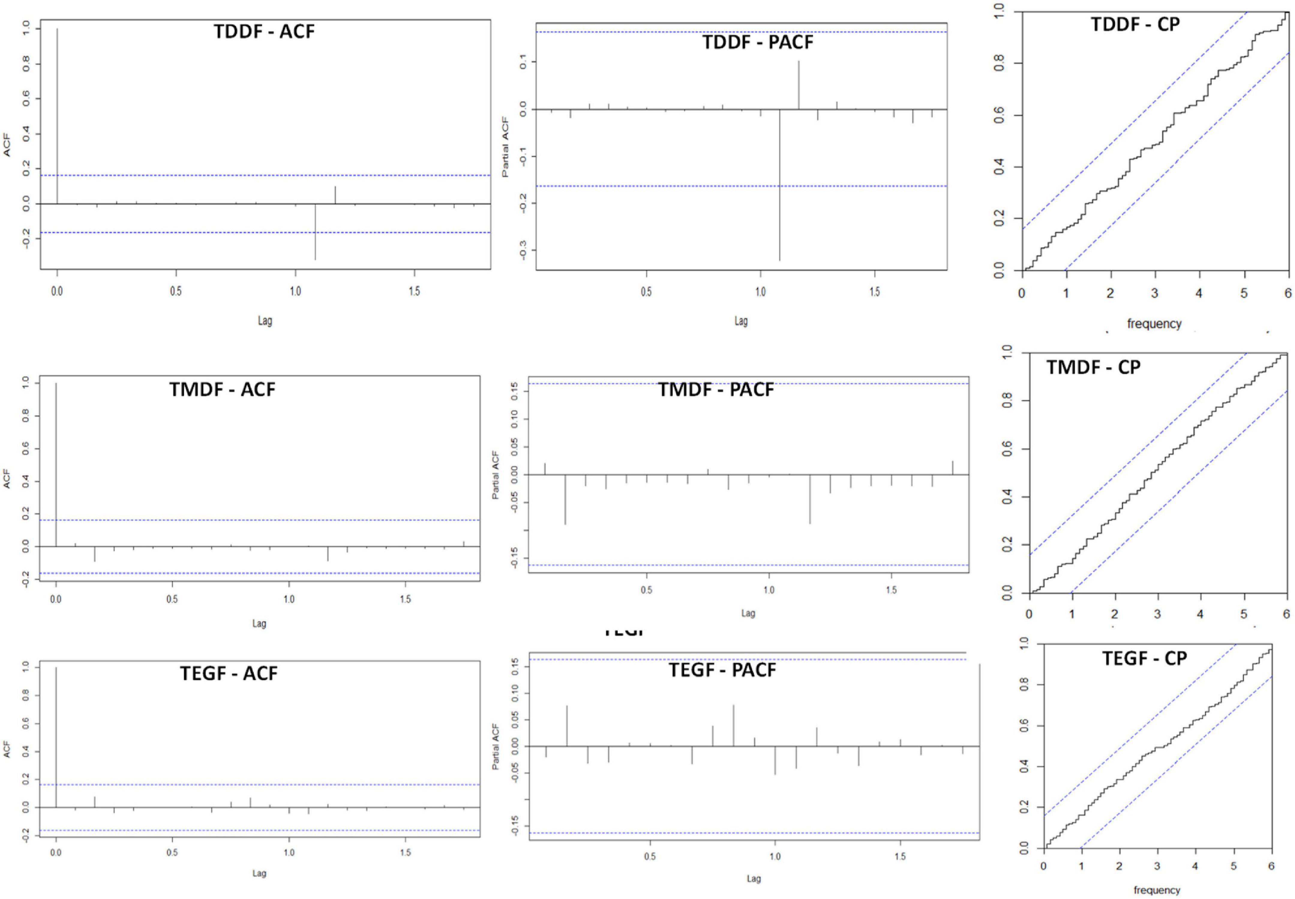
Figure 5. Residual ACF (autocorrelation function); PACF (partial autocorrelation function; CP (cumulative periodogram for TDDF (Tropical Dry Deciduous Forests, TMDF (Tropical Moist Deciduous Forest and TEGF (Tropical Evergreen Forests) for univariate ARIMA model.
The Portmanteau test (L-Jung box test) depicted that the residuals were not distinguishable from white noise, i.e., there was no serial correlation present (P > 0.05) (Table 1). Forecasting was carried out using “train” data (Figure 6). The plot of the forecasted and original fire depicted good agreement (Figure 7). There was, however, considerable variation between the original and forecasted values for TDDF during the year 2015, and the peak original fires were not in either 80 or 95% confidence bands. This was revived in 2016 and then in 2017. The TMDF exhibited good agreement between original and forecasted fires for the years 2015 and 2017; however, for 2017 a shift was observed during the peak fire months. The TEGF had a better agreement between original and forecasted fires in all the studied years. During the year 2017, however, there was over prediction of fire. The non-fire season active fire counts were in good agreement with forecasted fire for all the years and all the forest types.
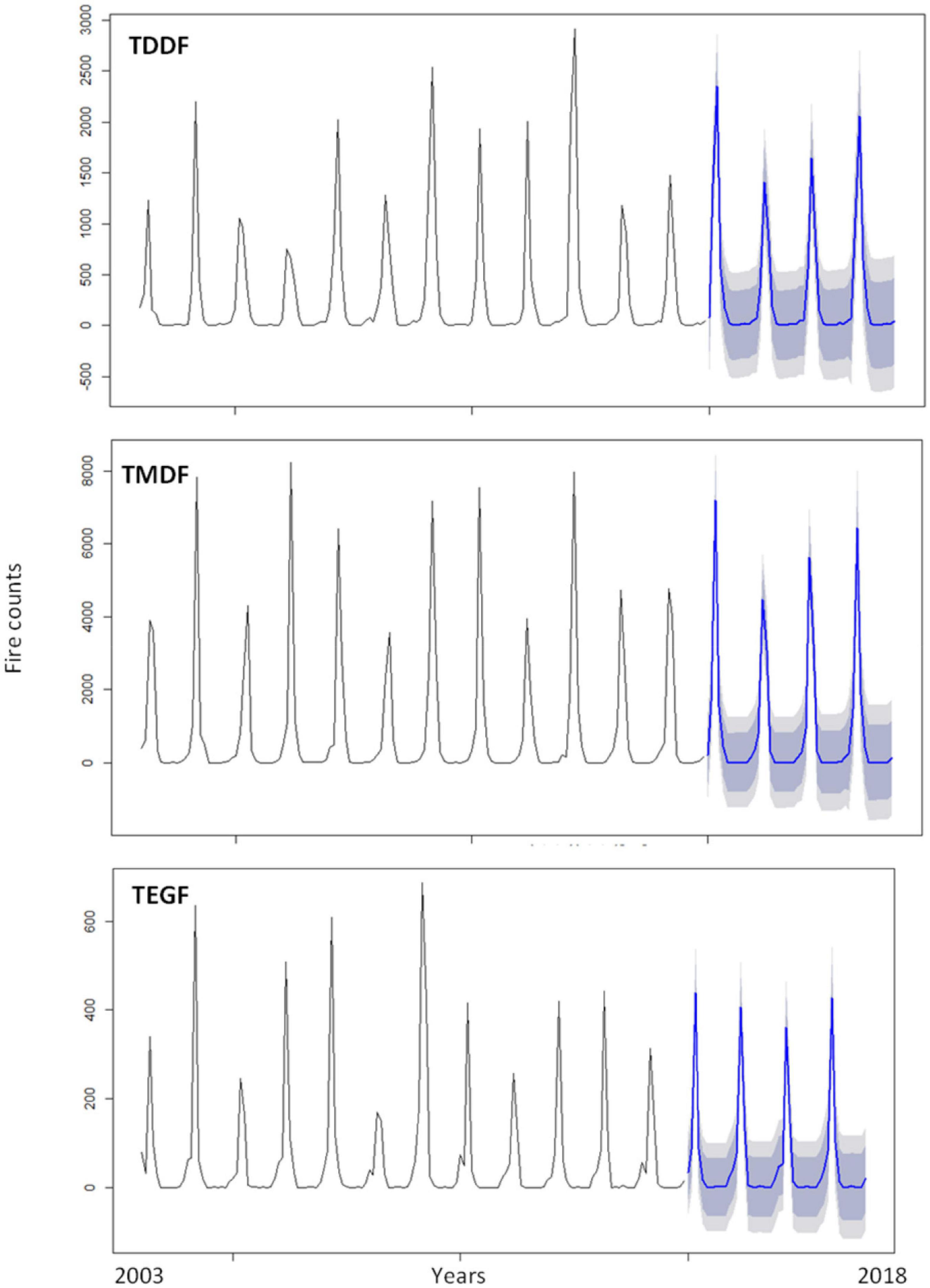
Figure 6. Forest fire forecasting based on ARIMA univariate model for Tropical Dry Deciduous Forests (TDDF) Tropical Moist Deciduous Forests (TMDF) and Tropical Evergreen Forests (TEGF). Blue lines depict forecasted fires and shaded area depicts prediction interval (inner to outer 80 and 95%, respectively).
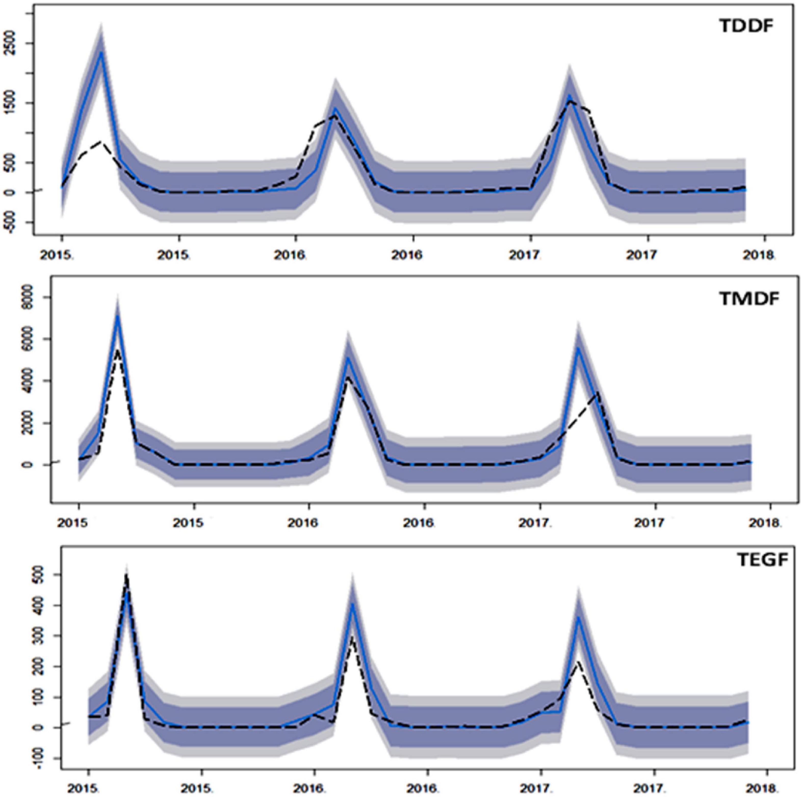
Figure 7. Comparison of ARIMA univariate model forecast, with test data (2015–2017) for Tropical Dry Deciduous Forests (TDDF) Tropical Moist Deciduous Forests (TMDF) and Tropical Evergreen Forests (TEGF). The dashed line depicts the original values, solid blue line depicts forecasted values and shaded area depicts prediction interval (inner to outer 80 and 95%, respectively).
ARIMA model with regressors considered temperature and dry days as independent variables. The p,d,q and P,D,Q-values for these forests types were,0,0,1 and 2,1,0 for TDDF; 2,0,0 and 2,1,1 for TMDF and 1,0,0 and 2,1, 0 for TEGF, respectively (Table 1 and Supplementary material 2). The residuals had insignificant autocorrelation and partial autocorrelation for all the forest types and the cumulative periodogram depicted insignificant periodicities (Figure 8). Portmanteau test also depicted that residual series was not distinguishable from white noise (Table 1).
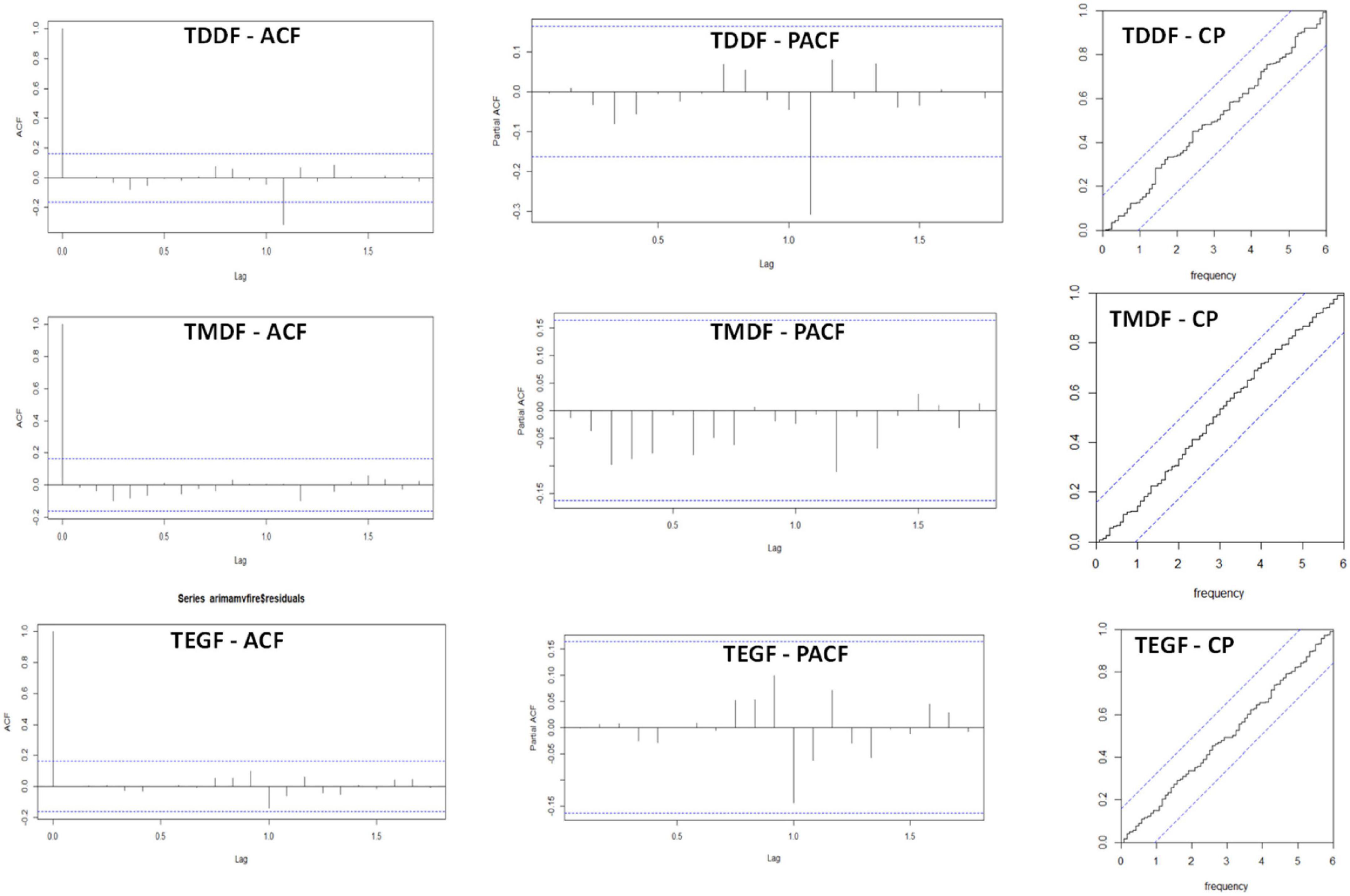
Figure 8. Residual Autocorrelation function (ACF), residual partial autocorrelation function (PACF) and cumulative periodogram (CP) of residual for ARIMA model with regressors (i.e., temperature and dry days) for Tropical Dry Deciduous Forests (TDDF) Tropical Moist Deciduous Forests (TMDF) and Tropical Evergreen Forests (TEGF).
Not much variation in R2 between original and forecasted forest fires was observed for the univariate ARIMA model and ARIMA model with regressors for all the forest types (Table 2). ARIMA model with regressors, however, had fluctuating minimum active fire counts during the non-fire season, which were smooth in the univariate model. This resulted in negative forecasted values (Figure 9). The overall trend of forecasted fire was more or less similar in both models (Figure 10).
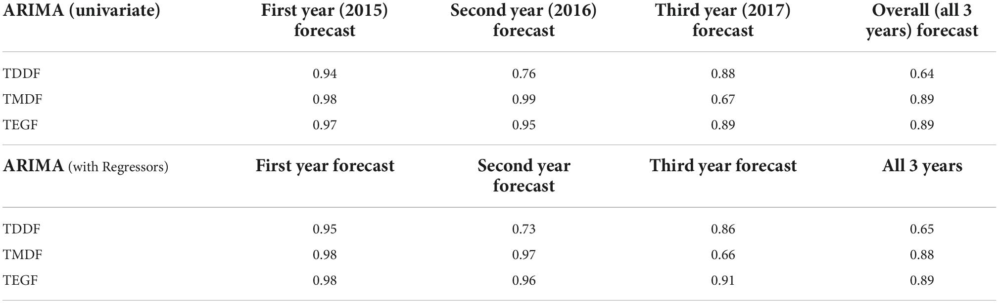
Table 2. Correlation [coefficient of determination (R2)] between original and forecasted monthly fire values from 2015 to 2017.
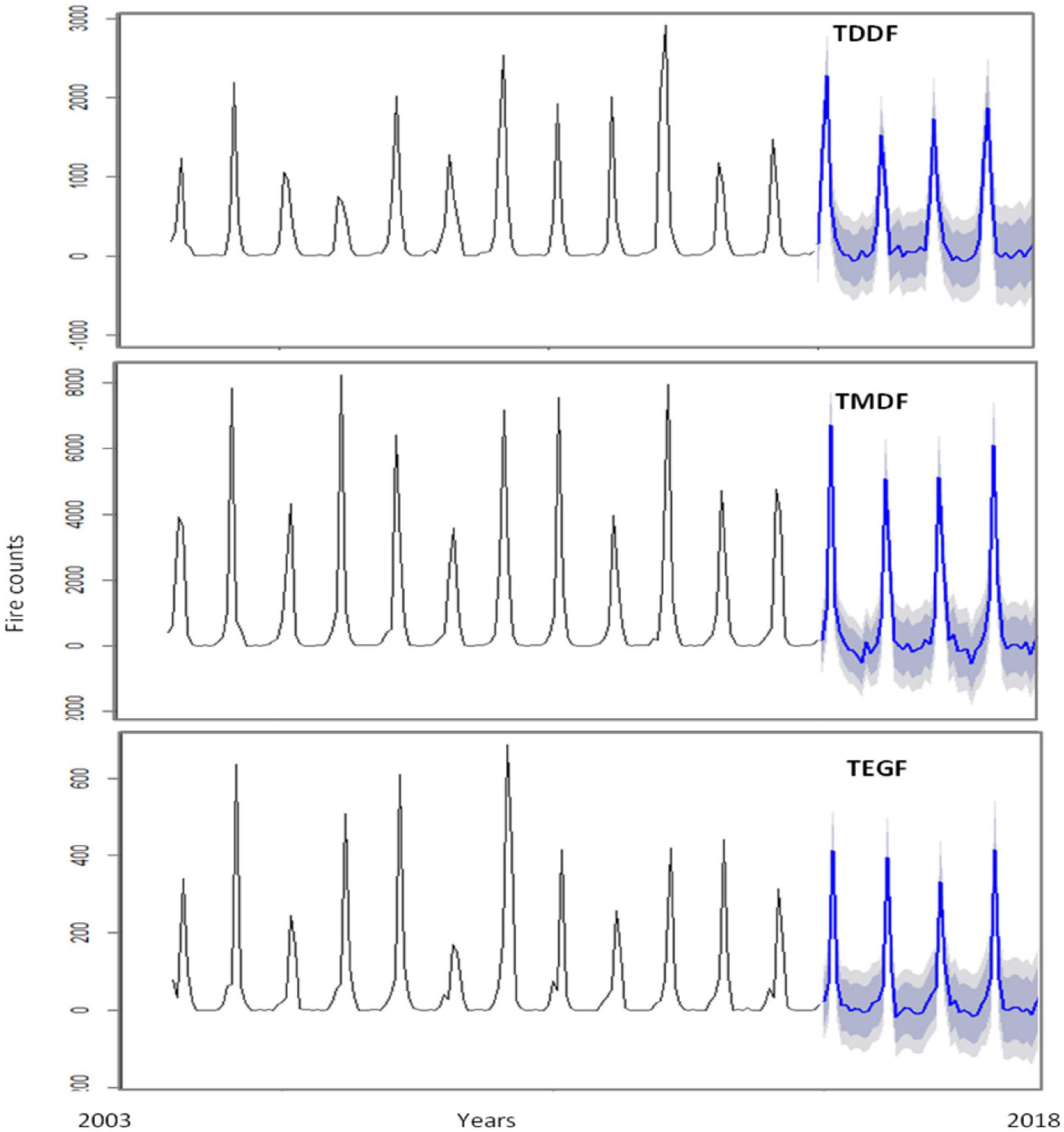
Figure 9. Forest fire forecasting based on ARIMA with regressors (temperature and dry days) model for Tropical Dry Deciduous Forests (TDDF), Tropical Moist Deciduous Forests (TMDF) and Tropical Evergreen Forests (TEGF). Blue lines depict forecasted fires and shaded area depicts prediction interval (inner to outer 80 and 95%, respectively).
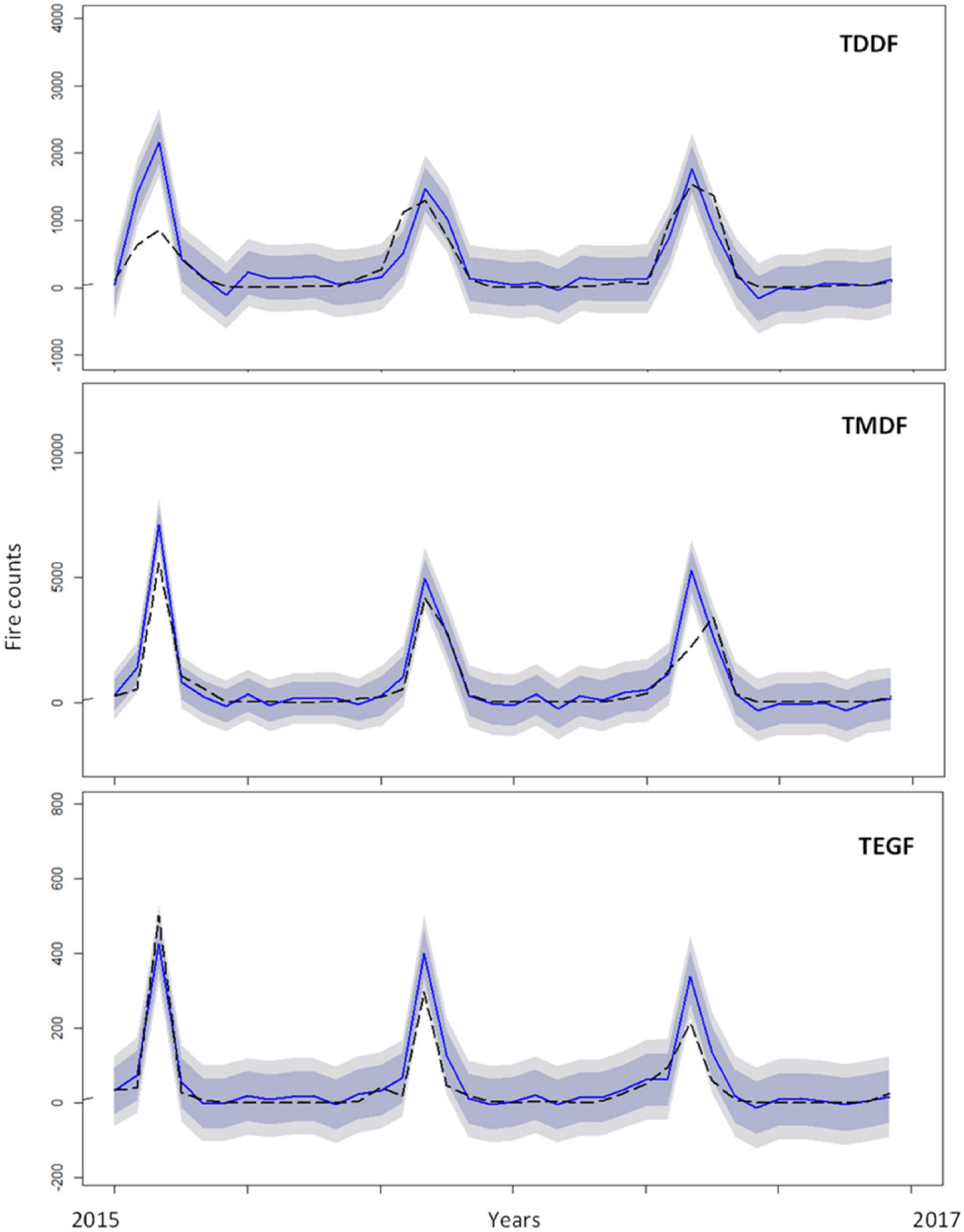
Figure 10. Comparison of ARIMA with regressors (temperature and dry days) model with test data (2015–2017) for Tropical Dry Deciduous Forests (TDDF), Tropical Moist Deciduous Forests (TMDF), Tropical Evergreen Forests (TEGF). The dotted line depict the original values, solid blue line depicts forecasted values and shaded area depicts prediction interval (inner to outer 80 and 95%, respectively).
On comparing the performance of the univariate ARIMA model and ARIMA model with regressors, no major difference was observed when overall model performance was concerned. A better agreement between forecasted and original active fire counts was observed for the year 1 for TDDF and TEGF when ARIMA model with regressors was used. For TMDF equal performance for year 1 was observed with both the models. Except for TDDF, the performance of both the models deteriorated from years 1 to 3. The agreement (R2) between the original and forecasted fires for the third year (2017) for TDDF and TMDF was superior in the univariate ARIMA model, whereas, for TEGF it was superior in the ARIMA model with regressors (Table 2). Among all the studied forests the third year (2017), forecast for TMDF was superior with the univariate model (Table 2).
Forest FFR provided information about fire susceptibility. For most of the forests, FFR ranged between 0 and 10. Higher FFR was depicted in the month of January, October, and December. North-East and Deccan Peninsula regions frequently depicted higher FFR in different months of the year. March and April were the prominent fire months; however, FFR did not increase significantly as the fire was well spread rather than clumped in specified regions. In May, FFR reduced in the central Deccan Peninsula and parts of North-East, which again increased in June in the central Deccan Peninsula. In October, high FFR was reported in the same region.
The original and forecasted FFRs were in good agreement for different months of the year 2017 (Figure 10). In March and May, there was underestimation of FFR in the central region of the Deccan peninsula, whereas, overestimation was observed in North-East in May. Some parts of the Deccan Peninsula had higher FFRs in October, which were also depicted in the forecasted FFR. In November, overestimation and in December underestimation were observed in the North-East region. For high and very high categories, original and forecasted FFRs were in good agreement (Figure 11). The FFRs were not forecasted for rainy season, i.e., July to September.
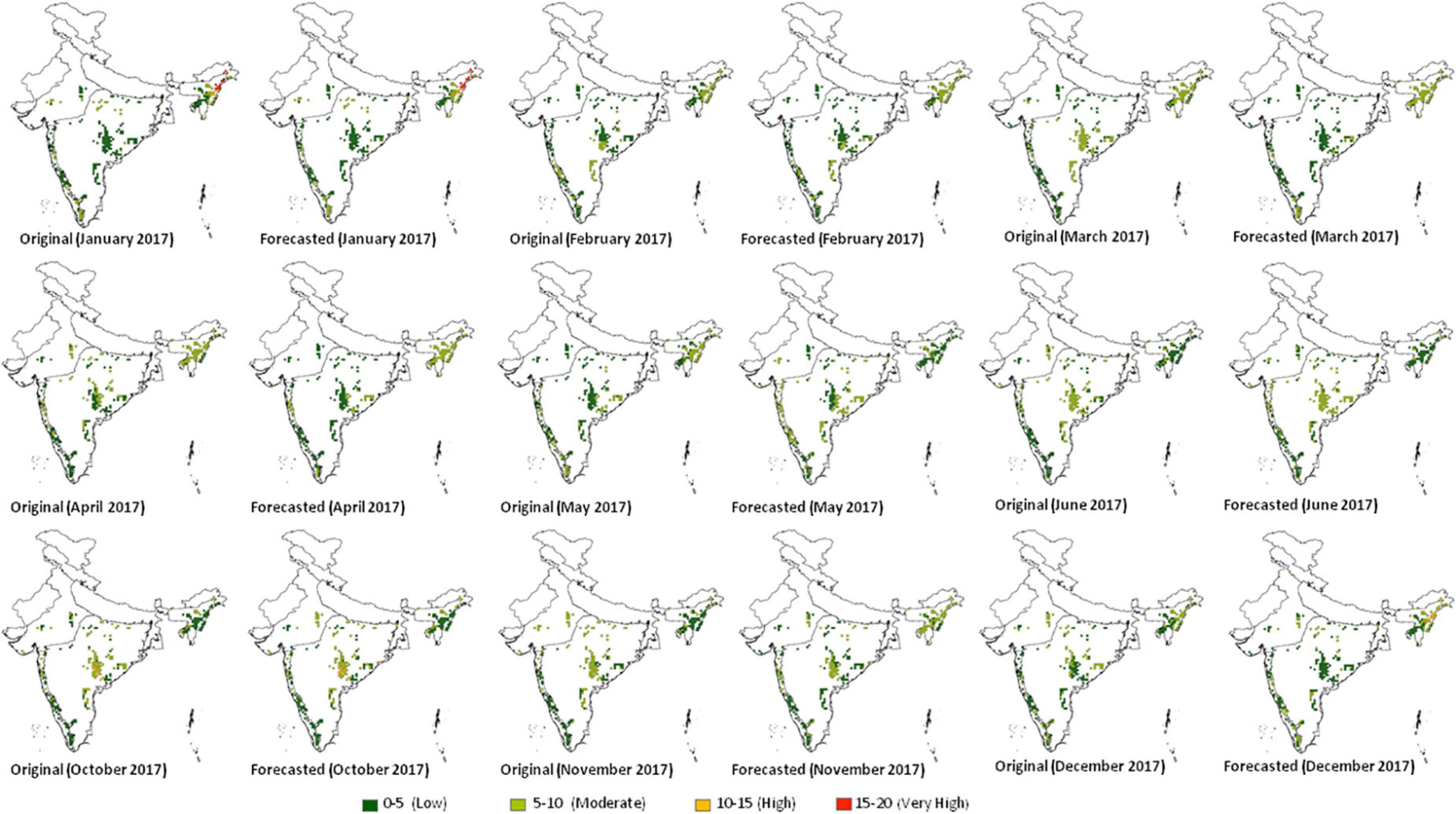
Figure 11. Original and forecasted forest fire frequency ratio (FFR) for January, February, March, April, May, June, October, November and December 2017 Biogeographic zone-wise (Rodgers and Panwar, 1988; Rodgers et al., 2000).
Discussion
The time series forecasting provides the flexibility to investigate the univariate as well as multivariate time series where the dynamic relationship of different variables are investigated. We investigated the univariate ARIMA model and ARIMA model with regressors. The univariate ARIMA is a single equation model which relates the future and past observations of a given time series, whereas, the ARIMA model with regressors is also a single equation model but also takes into consideration explanatory variables. It is based on the assumption that explanatory variables affect the response variables but not vice versa.
A multivariate ARIMA model is an n equation n variable linear model that relates to past values of different variables; thus, the variables relate dynamically in a closed loop system (Jones et al., 2009). As dry days and temperature used in the present study are causal variables of forest fire and vice versa is not true, i.e., forest fires do not cause variations in seasonal temperature and number of dry days (at least at regional scales), we found a single equation model with exogenous variable more appropriate for our research.
Even when multivariate time series models provide greater flexibility to investigate the dynamic relationships in different variables time series, on many occasions, it is practically difficult to find seamless data for multiple variables for a significant amount of time. This is where the univariate models are found useful as the data requirement is limited just to the single variable in question. As we had seamless time series available for dry days, temperature, and active fire, we experimented both with the univariate model and the model with regressors. We obtained near similar results with both the models and finally preferred the univariate model for forecasting forest fires considering the computational gains and parsimony. It would, however, be important to investigate the twofold modeling approach across different geographical set-ups to validate the findings of the present research.
It is worthwhile to argue for not using the ‘‘count’’ time series model even when the fire data was a ‘‘count’’ data. ‘‘Count’’ time series models are generally used for rare events. Typically, such models assume that the events are independent of time and thus they are memory-less.2 Wildfire has a well-defined seasonality in India. Further, the fire events are not “independent,” for example, during an extreme climate event, fire incidences are significant, but in the immediate next year fires are diminished mostly due to less availability of fuel (as it was consumed by fire in the previous year and could not be replenished through regeneration). It is therefore we preferred the regular ARIMA model to “count” time series models.
Some studies, for example by Albertson et al. (2009), used the probit model to consider the chance of wildfire breaking out on a given day. Such models are useful in predicting the presence or absence of fire on a given day. The authors could correctly predict five out of seven fires in a typical year. Our study was based on the monthly time series data, and hence such a model was of limited use; however, we believe that the model may be useful in estimating the probability of occurrence of fire on a particular day, i.e., on a holiday (as studied by the authors), particularly, in the set-up where forests have significant anthropogenic pressure. Kadir et al. (2020) used the ARIMA model to predict the hotspots in the Riau province of Indonesia. They could accurately forecast the hotspots for upto 5 months using the ARMA model. They have not used any explanatory variables for the occurrence of fire. We also believe that the univariate model may be extremely useful when monthly forest fire forecasting is the objective as the computation cost of regressors can be avoided. In the present research, the performance of univariate and model with regressors was near similar; however, for 1 year ahead, the forecast model with regressors was found slightly superior. The model with regressors may further be useful in studying the time series at weekly or daily time steps as the effect of climate variables on early or late occurrence of fire season can be studied objectively.
Viedma et al. (2018) used the longitudinal negative bionomial and the ZINB mixed models to model the number of fires. The main purpose of using these models was to handle the overdispersion (variance greater than the mean) or excess of 0 values present in the data. They experimented both with univariate as well as models involving explanatory variables. In the present research, no overdispersion or excess of 0 values was observed, and hence the ZINB model was not of much use.
Different studies have used auto.arima algorithm for the identification of the best ARIMA model for forecasting (Choudhary et al., 2022; Sharmin et al., 2022). Our study as well as the auto.arima algorithm worked well, and the p,d,q, and P,D,Q parameters obtained could provide a comparable active fire forecast with that of original active fire counts.
The fire forecast in the present research was based on 15 years of available active fire data from MODIS. During this time, forests owing to climate extremities encountered many fluctuations in fires, particularly in the years 2004, 2009, and 2012, thus the fire incidences considered in the present research were a mix of normal and extreme years, and no separate scenario was formed for normal and extreme years. This is justifiable because 1. Extreme events have become so frequent that they need to be included in TSA for meaningful forecasting and 2. It is important to consider all available data to have continuity in time series.
Biswas et al. (2015) found the fire susceptibility in Myanmar in the protected and non-protected areas and suggested that human activity explained most of the variance in burn probability. They suggested that fuel composition is one of the most important factors in determining fire susceptibility. Our study is in partial agreement with theirs. The forest fires in India are mainly anthropogenic. In some pockets of North-East India, shifting cultivation is a major driver of forest fires in the fire season. This has resulted in higher fire susceptibilities in these regions. We believe that climatic factors, i.e., temperature and dry days form conducive conditions for the fire to occur. It was observed that for lower FFRs, percent average contribution of vegetation type was maximum (25%), whereas, other causal drivers, i.e., elevation, slope, temperature, and dry days contributed 20, 22, 17, and 16%, respectively. As against this for higher FFRs, the temperature and dry days were the main causal drivers. In the month of January, the dry days and temperature together contributed around average 70% of the total FFR in the highest (15–20) FFR region. A similar trend was observed for all the months from February to April, which are the prominent fire months in India. This clearly indicates that the dry days and temperature are important fire drivers in India, and the forests remain less susceptible (despite the availability of fuel) to fire when these drivers are not significant contributors.
Among all the drivers studied, the average FFR from January to April (prominent fire months) was maximum for dry days followed by the slope. Except for elevation, all the drivers depicted decreasing trend from January to April and clumped around the value of 1 in the month of April. This indicates that during the start of the fire season, different drivers contribute maximum in defining the fire susceptibility, whereas, during the late fire season they have a minimum contribution.
In this research, we have explored the possibility of using FFR as an indicator by taking forecasted forest fires as the input. The forecasted active fire counts obtained were at the level of forest types and not at the level of 25 km × 25 km grid. This is because there may be instances when there are no incidences of fire at the grid level, thus the continuous data are not available, and the forecasting may not be meaningful.
We found both univariate ARIMA model and ARIMA model with regressors as potential tools to forecast forest fires. We preferred the univariate model due to parsimony. There is, however, a need to further investigate the model performance using high temporal and spatial resolution datasets.
The TSA is a data-intensive science, and better results are expected when fire data for a significant number of years is available. This also helps in validating the model with a larger test dataset. The correct MODIS active fire data is available since 2003 and there is a need to compile the forest fire data prior to 2003 from different available sources to further improve the forecasts.
Data availability statement
Publicly available datasets were analyzed in this study. This data can be found here: https://firms.modaps.eosdis.nasa.gov/download/.
Author contributions
All authors listed have made a substantial, direct, and intellectual contribution to the work, and approved it for publication.
Acknowledgments
We acknowledge the support received by P. Bhawani related to data format conversions.
Conflict of interest
The authors declare that the research was conducted in the absence of any commercial or financial relationships that could be construed as a potential conflict of interest.
Publisher’s note
All claims expressed in this article are solely those of the authors and do not necessarily represent those of their affiliated organizations, or those of the publisher, the editors and the reviewers. Any product that may be evaluated in this article, or claim that may be made by its manufacturer, is not guaranteed or endorsed by the publisher.
Supplementary material
The Supplementary Material for this article can be found online at: https://www.frontiersin.org/articles/10.3389/ffgc.2022.882685/full#supplementary-material
Footnotes
References
Albertson, K., Aylen, J., Cavan, G., and Mcmorrow, J. (2009). Forecasting the outbreak of moorland wildfires in the English Peak district. J. Environ. Manage. 90, 2642–2651. doi: 10.1016/j.jenvman.2009.02.011
Aldersley, A., Murray, S. J., and Cornell, S. E. (2011). Global and regional analysis of climate and human drivers of wildfire. Sci. Total. Environ. 409, 3472–3481. doi: 10.1016/j.scitotenv.2011.05.032
Allexander, J. D., Seavy, N. E., Ralph, C. J., and Hogoboom, B. (2006). Vegetation and topographical correlates of fire severity from two fire in the Klamath-Siskiyou region of Oregon and California. Int. J. Wildland Fire 15, 237–245. doi: 10.1071/WF05053
Biswas, S., Vadrevu, K. P., Lwin, Z. M., Lasko, K., and Justice, C. O. (2015). Factors controlling vegetation fires in protected and non-protected areas of Myanmar. PLoS One 10:e0124346. doi: 10.1371/journal.pone.0124346
Bond, W. J., and Keeley, J. E. (2005). Fire as a global herbivore: The ecology and evolution of flammable ecosystems. Trends Ecol. Evol. 20, 387–394. doi: 10.1016/j.tree.2005.04.025
Bowman, D. M., Balch, J., Artaxo, P., Bond, W. J., Cochrane, M. A., D’antonio, C. M., et al. (2011). The human dimension of fire regimes on Earth. J. biogeogr. 38, 2223–2236. doi: 10.1111/j.1365-2699.2011.02595.x
Bowman, D., Williamson, G., Yebra, M., Loila, J. L., Pettinari, M. L., Shah, S., et al. (2020). Wildfires: Australia needs a national monitoring agency. Nature 584, 118–191. doi: 10.1038/d41586-020-02306-4
Box, G. E. P., and Pierce, D. A. (1970). Distribution of residual correlations in autoregressive-integrated moving average time series models. J. Am. Stat. Assoc. 65, 1509–1526. doi: 10.2307/2284333
Briët, O. J., Amerasinghe, P. H., and Vounatsou, P. (2013). Generalized seasonal autoregressive integrated moving average models for count data with application to malaria time series with low case numbers. PLoS One 8:e65761. doi: 10.1371/journal.pone.0065761
Champion, H. G., and Seth, S. K. (2005). A revised survey of the forest types of India. Dehradun: Natraj Public.
Choudhary, A., Kumar, S., Sharma, M., and Sharma, K. P. (2022). A framework for data prediction and forecasting in WSN with Auto ARIMA. Wireless. Pers. Commun. 123, 2245–2259. doi: 10.1007/s11277-021-09237-x
Coghlan. (2018). A little book of R for time series release 0.2. Available online at: https://buildmedia.readthedocs.org/media/pdf/a-little-book-of-r-for-time-series/latest/a-little-book-of-r-for-time-series.pdf (accessed February 10, 2022).
Contreras, J., Espinola, R., Nogales, F. J., and Conejo, A. J. (2003). ARIMA models to predict next-day electricity prices. IEEE Trans. Power Syst. 18:3. doi: 10.1109/TPWRS.2002.804943
Devischer, T., Anderson, L. O., Aragao, L., Galvan, L., and Malhi, Y. (2016). Increased wildfire risk driven by climate and development interactions in the bolivian chiquitania, Southern Amazonia. PLoS One 11:e0161323. doi: 10.1371/journal.pone.0161323
Du, H., Nguyen, L., Yang, Z., Gellban, H. A., Zhou, X., Xing, W., et al. (2019). “Twitter vs news: Concern analysis of the 2018 California wildfire event,” in Proceedings of the IEEE 43rd annual computer software and applications conference (COMPSAC), Milwaukee, WI. doi: 10.1109/COMPSAC.2019.10208
EARTHDATA (2022). Fire information for resource management system (FIRMS). Available online at: https://earthdata.nasa.gov/earth-observation-data/near-real-time/firms (accessed January 14, 2022).
EFFIS (2022). European forest fire information system. Available online at: https://effis.jrc.ec.europa.eu. (accessed September 03, 2022).
Feng, L., and Shi, Y. (2018). Forecasting mortality rates: Multivariate or univariate models? J. Pop. Res. 35, 289–318. doi: 10.1007/s12546-018-9205-z
Freifelder, R. R., Vitousek, P. M., and D’antonio, C. M. (1998). Microclimate change and effect on fire following forest-grass conversion in seasonally dry tropical woodland. Biotropica 30, 286–297. doi: 10.1111/j.1744-7429.1998.tb00062.x
FSI (2022). FSI forest fire alert system (FAST 3.0). Available online at: http://fsi.nic.in/uploads/documents/technical_information_series_vol1_no2.pdf (accessed January 14, 2022)
Giannaros, T. M., Lagouvardos, K., and Kotroni, V. (2020). Performance evaluation of an operational rapid response fire spread forecasting system in the southeast mediterranean (Greece). Atmosphere 11:1264. doi: 10.3390/atmos11111264
Graff, C. A., Coffield, S. R., Chen, Y., Georgiou, E. F., Randerson, J. T., and Smyth, P. (2020). Forecasting daily wildfire activity using poisson regression. IEEE Trans. Geosci. Remote Sens. 58:7. doi: 10.1109/TGRS.2020.2968029
Huesca, M., Litago, J., Miguel, S., Ocana, V., and Orueta, A. (2014). Modeling and forecasting MODIS-based Fire Potential Index on a pixel basis using time series models. Int. J. Appl. Earth Obs. Geoinf. 26, 363–376. doi: 10.1016/j.jag.2013.09.003
Hyndman, R. J. (2022b). Forecasting: Principles and practice, dynamic regression. Available online at: https://robjhyndman.com/acemsforecasting2018/3-Dynamic-Regression.pdf (Accessed August 27, 2022).
Hyndman, R. J. (2022a). Facts and fallacies of AIC. Available online at: https://robjhyndman.com/hyndsight/aic/ (accessed February 11, 2022).
Hyndman, R. J., and Athanasopoulos, G. (2018). Forecasting: Principles and practice, 2nd Edn. Melbourne: OTexts.
Hyndman, R. J., and Khandakar, Y. (2008). Automatic time series forecasting: The forecast package for R. J. Stat. Soft. 27, 1–22. doi: 10.18637/jss.v027.i03
Hyndman, R., Athanasopoulos, G., Bergmeir, C., et al. (2022). Forecasting functions for time series and linear models. Available online at: https://cran.r-project.org/web/packages/forecast/forecast.pdf (accessed August 17, 2022).
Iwok, I. A., and Okpe, A. S. (2016). A comparative study between univariate and multivariate linear stationary time series models. Am. J. Math. Stat. 6, 203–212.
Jesus, C. S. L., Delgado, R. C., Wanderley, H. S., Teodoro, P. E., Pereria, M. G., Lima, M., et al. (2022). Fire risk associated with landscape changes, climatic events and remote sensing in the Atlantic forest using ARIMA model. Remote Sens. Appl. Soc. Environ. 26:100761. doi: 10.1016/j.rsase.2022.100761
Jha, C. S., Gopalkrishnan, R., Thumaty, K. C., Singhal, J., Reddy, C. S., Singh, J., et al. (2016). Monitoring of forest fires from space – ISRO’s initiative for near real-time monitoring of the recent forest fires in Uttarakhand, India. Curr. Sci. 110, 2057–2060.
Jones, S. S., Evans, R. S., Allen, T. L., Thomas, A., Haug, P. J., Welch, S. J., et al. (2009). A multivariate time series approach to modeling and forecasting demand in the emergency department. J. Biomed. Inform. 42, 123–139. doi: 10.1016/j.jbi.2008.05.003
Kadir, E. A., Dayana, N. E., Rosa, S. L., Othman, M., and Saian, R. (2020). Prediction of hotspots in riau province, indonesia using the autoregressive integrated moving average (ARIMA) model. SAR J. 3, 101–110. doi: 10.18421/SAR33-03
Kale, M. P., Ramachandran, R. M., Pardeshi, S. N., Chavan, M., Joshi, P. K., Pai, D. S., et al. (2017). Are climate extremities changing forest-fire regimes in India? An analysis using MODIS fire locations of 2003-2013 and gridded climate data of India meteorological department. Proc. Natl. Acad. Sci. Ind. 87, 827–843. doi: 10.1007/s40010-017-0452-8
Kashyap, R. L., and Rao, A. R. (1976). Dynamic stochastic models from empirical data. New York, NY: Academic Press.
Kidzberger, T., Brown, P. M., Heyerdahl, E. K., Swetnam, T. W., and Veblen, T. T. (2007). Contingent Pacific–Atlantic Ocean influence on multicentury wildfire synchrony over western North America. Proc. Natl. Acad. Sci. 104, 543–548. doi: 10.1073/pnas.0606078104
Kodandpani, N., Cochrane, M. A., and Sukumar, R. (2008). A comparative analysis of spatial, temporal, and ecological characteristics of forest fires in seasonally dry tropical ecosystems in the Western Ghats, India. For. Ecol. Manage. 256, 607–617. doi: 10.1016/j.foreco.2008.05.006
Laurance, W. F., Goosem, M., and Laurance, S. G. W. (2009). Impacts of roads and linear clearings on tropical forests. Trends. Ecol. Evol. 24, 659–669. doi: 10.1016/j.tree.2009.06.009
Lee, S., and Pradhan, B. (2007). Landslide hazard mapping at Selangor, Malaysia using frequency ratio and logistic regression models. Landslides 4, 33–41. doi: 10.1007/s10346-006-0047-y
Lei, S. D. (2017). Predict the future hospitalized patients number based on patient’s temporal and spatial fluctuations using a hybrid ARIMA and wavelet transform model. J. Geog. Inf. Syst. 9, 456–465. doi: 10.4236/jgis.2017.94028
Ljung, G., and Box, G. E. P. (1978). On a measure of lack of fit in time series models. Biometrika. 65, 297–303. doi: 10.2307/2335207
Mandel, J., Amram, S., Beezley, J. D., Kelman, G., Kochanski, A. K., Kondratenko, V. Y., et al. (2014). New features in WRF-SFIRE and the wildfire forecasting and danger system in Israel. Nat. Hazards Earth Syst. Sci. Discuss. 2, 1759–1797. doi: 10.5194/nhessd-2-1759-2014
McKenzie, D., Gedalof, Z., Peterson, D. L., and Mote, P. (2004). Climatic change, wildfire, and conservation. Conserv. Biol. 18, 890–902. doi: 10.1111/j.1523-1739.2004.00492.x
Michael, Y., Helman, D., Glickman, O., Gabay, D., Brenner, S., and Lensky, I. M. (2021). Forecasting fire risk with machine learning and dynamic information derived from satellite vegetation index time-series. Sci. Total Envion. 764:142844. doi: 10.1016/j.scitotenv.2020.142844
MODIS (2022). Modis active fire and burned area products. Available online at: https://modis-fire.umd.edu (accessed January 15, 2022).
Mujumdar, P. P. (2022). Time series analysis. Available online at: https://nptel.ac.in/courses/105/108/105108079/#, (accessed February 11, 2022).
Mujumdar, P. P., and Kumar, D. N. (1990). ‘Stochastic models of streamflow: Some case studies’. Hydrol. Sci. J. 35, 395–410. doi: 10.1080/02626669009492442
N’Datchoh, E. T., Konare, A., Diedhiou, A., Diawra, A., Quansah, E., and Assamoi, P. (2015). Effects of climate variability on Savannah fire regimes in West Africa. Earth Syst. Dyn. 6, 161–174. doi: 10.5194/esd-6-161-2015
Natural Resource Canada (2022). Available online at: https://cwfis.cfs.nrcan.gc.ca/maps/fw?type=ffmc&year=2022&month=2&day=19 (accessed February 18, 2022).
NAU (2020). Statistical forecasting: Notes on regression and time series analysis. Available online at: https://people.duke.edu/~rnau/411home.htm (accessed February 10, 2022).
Pai, D. S., Sridhar, L., Rajeevan, M., Sreejith, O. P., Satbhai, N. S., and Mukhopadhyay, B. (2014). Development of a new high spatial resolution (0.25°× 0.25°) long period (1901–2010) daily gridded rainfall data set over India and its comparison with existing data sets over the region. Mausam 65, 1–18. doi: 10.54302/mausam.v65i1.851
Patra, P. K., Ishizawa, M., Maksyutov, S., Nakazawa, T., and Inoue, G. (2005). Role of biomass burning and climate anomalies for land–atmosphere carbon fluxes based on inverse modelling of atmospheric CO2. Glob. Biogeochem. Cycles 19:GB3005. doi: 10.1029/2004GB002258
Pradhan, B. (2010). Landslide susceptibility mapping of a catchment area using frequency ratio, fuzzy logic and multivariate logistic regression approaches. J. Indian Soc. Remote Sens. 38, 301–320. doi: 10.1007/s12524-010-0020-z
Preez, J. D., and Witt, S. F. (2003). Univariate versus multivariate time series forecasting: An application to international tourism demand. Int. J. Forecast. 19, 435–451. doi: 10.1016/S0169-2070(02)00057-2
Preisler, H. K., and Westerling, A. L. (2007). Statistical model for forecasting monthly large wildfire events in Western united states. J. Appl. Meteorol. Climatol. 46, 1020–1030. doi: 10.1175/JAM2513.1
Prestemon, J. F., Chas-Amil, M. L., Touza, J. M., and Goodrick, S. L. (2012). Forecasting intentional wildfires using temporal and spatiotemporal autocorrelations. Int. J. Wildland Fire 21, 743–754. doi: 10.1071/WF11049
Reilly, M. J., Dunn, C. J., Meigs, G. W., Spies, T. A., Kennedy, R. E., Bailey, J. D., et al. (2017). Contemporary patterns of fire extent and severity in forests of the Pacific Northwest, USA (1985–2010). Ecosphere 8:e01695. doi: 10.1002/ecs2.1695
Rodgers, W. A., and Panwar, H. S. (1988). Biogeographical classification of India. Dehradun: Wildlife Institute of India.
Rodgers, W. A., Panwar, H. S., and Mathur, V. B. (2000). Wildlife protected area network in India: A review, executive summary. Dehradun: Wildlife Institute of India.
Rodrigues, M., de la Riva, J., and Fotheringham, S. (2014). Modeling the spatial variation of the explanatory factors of human-caused wildfires in Spain using geographically weighted logistic regression. Appl. Geogr. 48, 52–63. doi: 10.1016/j.apgeog.2014.01.011
Rollins, M. G., Morgan, P., and Swetnam, T. (2002). Landscape-scale controls over 20th century fire occurrence in two large rocky mountain (USA) wilderness areas. Landscape Ecol. 17, 539–557. doi: 10.1023/A:1021584519109
Roy, P. S., Behera, M. D., Murthy, M. S. R., Roy, A., Singh, S., Kushwaha, S. P. S., et al. (2015). New vegetation type map of India prepared using satellite remote sensing: Comparison with global vegetation maps and utilities. Int. J. Appl. Earth Obs. Geoinf. 39, 142–159. doi: 10.1016/j.jag.2015.03.003
Salles, R. P., and Ogasawara, E. (2022). TSPred package for R : Framework for nonstationary time series prediction. Available online at: https://github.com/RebeccaSalles/TSPred/wiki (accessed January 24, 2022). doi: 10.1016/j.neucom.2021.09.067
Santana, N. C., Carvalho Junior, O., Gomes, R. A., and Guimaraes, R. F. (2018). Burned-area detection in amazonian environments using standardized time series per pixel in MODIS data. Remote Sens. 10:1904. doi: 10.3390/rs10121904
Sarfo, P. A., Mai, Q., Sanfilippo, F. M., Preen, D. B., Stewart, L. M., and Fatovich, D. M. (2015). A comparison of multivariate and univariate time series approaches to modelling and forecasting emergency department demand in Western Australia. Aust. J. Biomed. Informatics 57, 62–73. doi: 10.1016/j.jbi.2015.06.022
Satendra Kaushik, A. D. (2014). Forest fire diaster management. New Delhi: National Institute of Disaster Management, Ministry of Home Affairs.
Sethi, J. K., and Mittal, M. (2020). “Analysis of air quality using univariate and multivariate time series models,” in Proceedings of the 10th international conference on cloud computing, data science & engineering (Confluence), Noida, 823–827. doi: 10.1109/Confluence47617.2020.9058303
Sharmin, S., Alam, F. I., Das, A., and Uddin, R. (2022). “An investigation into crime forecast using auto ARIMA and stacked LSTM,” in Proceedings of the 2022 international conference on innovations in science, engineering and technology (ICISET), Chittagong, 415–420. doi: 10.1109/ICISET54810.2022.9775862
Siegert, F., and Hoffmann, A. A. (2000). The 1998 forest fires in East Kalimantan (Indonesia): A quantitative evaluation using high resolution, multitemporal ERS-2 SAR images and NOAA-AVHRR hotspot data. Remote Sens. Environ. 72, 64–77. doi: 10.1016/S0034-4257(99)00092-9
Siegert, F., Ruecker, G., Hinrichs, A., and Hoffmann, A. A. (2001). Increased damage from fires in logged forests during droughts caused by El Niño. Nature 414, 437–440. doi: 10.1038/35106547
Singleton, M. P., Thode, A. E., Meador, A. J. S., and Iniguez, J. M. (2019). Increasing trends in high-severity fire in the south western USA from 1984 to 2015. For. Ecol. Manag. 433, 709–719. doi: 10.1016/j.foreco.2018.11.039
Sivrikaya, F., and Kucuk, O. (2021). Modeling forest fire risk based on GIS-based analytical hierarchy process and statistical analysis in Mediterranean region. Ecol. Inf. 68:101537. doi: 10.1016/j.ecoinf.2021.101537
Slavia, A. P., Sutoyo, E., and Witarsyah, D. (2019). “Hotspots forecasting using autoregressive integrated moving average (ARIMA) for detecting forest fires,” in Proceedings of the IEEE international conference on internet of things and intelligence system (IoTaIS), Bali. doi: 10.1109/IoTaIS47347.2019.8980400
Srivastava, A. K., Rajeevan, M., and Kshirsagar, S. R. (2009). Development of a high resolution daily gridded temperature dataset (1969–2005) for the Indian region. Atmos. Sci. Lett. 10, 249–254. doi: 10.1002/asl.232
STACKOVERFLOW (2022). ARIMA forecasting with auto.Arima() and xreg. Available online at: https://stackoverflow.com/questions/34249477/arima-forecasting-with-auto-arima-and-xreg (accessed February 10, 2022).
Suresh, H. S., Dattaraja, H. S., and Sukumar, R. (1996). The flora of Mudumalai wildlife sanctuary, Tamil Nadu, southern India. Indian For. 122, 507–519.
UCAR (2022). Coupled weather – fire modeling. Available online at: https://ral.ucar.edu/wsap/coupled-weather-fire-modeling (accessed August 19 2022).
Urbieta, I. R., Franquesa, M., Veidma, O., and Moreno, J. M. (2019). Fire activity and burned forest lands decreased during the last three decades in Spain. Ann. For. Sci. 76:90. doi: 10.1007/s13595-019-0874-3
USDA (2022). National fire danger rating system. Available online at: https://www.fs.usda.gov/detail/cibola/landmanagement/resourcemanagement/?cid=stelprdb5368839 (accessed February 18, 2022)
Viedma, O., Urbieta, I. R., and Moreno, J. M. (2018). Wildfres and the role of their drivers are changing over time in a large rural area of west-central Spain. Sci. Rep. 8:17797. doi: 10.1038/s41598-018-36134-4
Walters, T. (2022). Time series analysis in R part 1: The time series object. Available online at: https://datascienceplus.com/time-series-analysis-in-r-part-1-the-time-series-object/ (accessed February 10, 2022).
Wangdi, K., Singhasivanon, P., Silawan, T., Lawpoolsri, S., White, N. J., and Kaewkungwal, J. (2010). Development of temporal modelling for forecasting and prediction of malaria infections using time-series and ARIMAX analyses: A case study in endemic districts of Bhutan. Malar. J. 9:251. doi: 10.1186/1475-2875-9-251
Westerling, A. L., Gershunov, A., Cayan, D. R., and Barnett, T. P. (2002). Long lead statistical forecasts of area burned in western US wildfires by ecosystem province. Int. J. Wildland Fire 11, 257–266. doi: 10.1071/WF02009
Woods, P. (1989). Effects of logging drought and fire on structure and composition of tropical forests in Sabah, Malaysia. Biotropica 21, 290–298. doi: 10.2307/2388278
Ye, T., Wang, Y., Guo, Z., and Li, Y. (2017). Factor contribution to fire occurrence, size, and burn probability in a subtropical coniferous forest in East China. PLoS One 12:e0172110. doi: 10.1371/journal.pone.0172110
Zhang, X., Zhang, T., Pei, J., Liu, Y., Li, X., and Gracia, P. M. (2016). Time series modelling of syphilis incidence in China from 2005 to 2012. PLoS One 11:e0149401. doi: 10.1371/journal.pone.0149401
Keywords: forecasting, ARIMA, wildfire, time series, fire alert, forest, frequency ratio, satellite remote sensing
Citation: Kale MP, Mishra A, Pardeshi S, Ghosh S, Pai DS and Roy PS (2022) Forecasting wildfires in major forest types of India. Front. For. Glob. Change 5:882685. doi: 10.3389/ffgc.2022.882685
Received: 24 February 2022; Accepted: 28 September 2022;
Published: 25 October 2022.
Edited by:
Giuseppe Ruello, University of Naples Federico II, ItalyReviewed by:
Marcos Rodrigues, University of Zaragoza, SpainItziar R. Urbieta, University of Castilla-La Mancha, Spain
Copyright © 2022 Kale, Mishra, Pardeshi, Ghosh, Pai and Roy. This is an open-access article distributed under the terms of the Creative Commons Attribution License (CC BY). The use, distribution or reproduction in other forums is permitted, provided the original author(s) and the copyright owner(s) are credited and that the original publication in this journal is cited, in accordance with accepted academic practice. No use, distribution or reproduction is permitted which does not comply with these terms.
*Correspondence: Manish P. Kale, manishk@cdac.in
†These authors have contributed equally to this work
‡These authors share senior authorship
§ORCID: Parth Sarathi Roy, orcid.org/0000-0002-6803-6785